Algorithmic Value Oscillator [CRYPTIK1]Algorithmic Value Oscillator
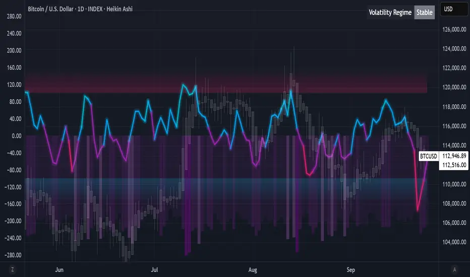
Introduction: What is the AVO? Welcome to the Algorithmic Value Oscillator (AVO), a powerful, modern momentum indicator that reframes the classic "overbought" and "oversold" concept. Instead of relying on a fixed lookback period like a standard RSI, the AVO measures the current price relative to a significant, higher-timeframe Value Zone .
This gives you a more contextual and structural understanding of price. The core question it answers is not just "Is the price moving up or down quickly?" but rather, " Where is the current price in relation to its recently established area of value? "
This allows traders to identify true "premium" (overbought) and "discount" (oversold) levels with greater accuracy, all presented with a clean, futuristic aesthetic designed for the modern trader.
The Core Concept: Price vs. Value The market is constantly trying to find equilibrium. The AVO is built on the principle that the high and low of a significant prior period (like the previous day or week) create a powerful area of perceived value.
The Value Zone: The range between the high and low of the selected higher timeframe.
Premium Territory (Distribution Zone): When the oscillator moves into the glowing pink/purple zone above +100, it is trading at a premium.
Discount Territory (Accumulation Zone): When the oscillator moves into the glowing teal/blue zone below -100, it is trading at a discount.
Key Features
1. Glowing Gradient Oscillator: The main oscillator line is a dynamic visual guide to momentum.
The line changes color smoothly from light blue to neon teal as bullish momentum increases.
It shifts from hot pink to bright purple as bearish momentum increases.
Multiple transparent layers create a professional "glow" effect, making the trend easy to see at a glance.
2. Dynamic Volatility Histogram: This histogram at the bottom of the indicator is a custom volatility meter. It has been engineered to be adaptive, ensuring that the visual differences between high and low volatility are always clear and dramatic, no matter your zoom level. It uses a multi-color gradient to visualize the intensity of market volatility.
3. Volatility Regime Dashboard: This simple on-screen table analyzes the histogram and provides a clear, one-word summary of the current market state: Compressing, Stable, or Expanding.
How to Use the AVO: Trading Strategies
1. Reversion Trading This is the most direct way to use the indicator.
Look for Buys: When the AVO line drops into the teal "Accumulation Zone" (below -100), the price is trading at a discount. Watch for the oscillator to form a bottom and start turning up as a signal that buying pressure is returning.
Look for Sells: When the AVO line moves into the pink "Distribution Zone" (above +100), the price is trading at a premium. Watch for the oscillator to form a peak and start turning down as a signal that selling pressure is increasing.
2. Best Practices & Settings
Timeframe Synergy: The AVO is most effective when your chart timeframe is lower than your selected "Value Zone Source." For example, if you trade on the 1-hour chart, set your Value Zone to "Previous Day."
Confirmation is Key: This indicator provides powerful context, but it should not be used in isolation. Always combine its readings with your primary analysis, such as market structure and support/resistance levels.
M-oscillator
Premier Stochastic Oscillator [LazyBear, V2]This script builds on the well-known Premier Stochastic Oscillator (PSO) originally introduced by LazyBear, and adds a Z-Score extension to provide statistical interpretation of momentum extremes.
Features
Premier Stochastic Core: A smoothed stochastic calculation that highlights bullish and bearish momentum phases.
Z-Score Mapping: The PSO values are standardized into Z-Scores (from –3 to +3), quantifying the degree of momentum stretch.
Positive / Negative Z-Scores:
Positive Z values suggest momentum strength that can align with accumulation or favorable buying conditions.
Negative Z values indicate stronger bearish pressure, often aligning with selling or distribution conditions.
On-Chart Label: The current Z-Score is displayed on the latest bar for quick reference.
How to Use
Momentum Confirmation: Use the oscillator to confirm whether bullish or bearish momentum is intensifying.
Overextended Conditions: Extreme Z-Scores (±2 or beyond) highlight statistically stretched conditions, often preceding reversions.
Strategic Integration: Best applied in confluence with trend tools or higher-timeframe filters; not a standalone trading signal.
Originality
Unlike the standard PSO, this version:
Adds a Z-Score framework for objective statistical scaling.
Provides real-time labeling of Z values for clarity.
Extends the classic oscillator into a tool for both momentum detection and mean-reversion context.

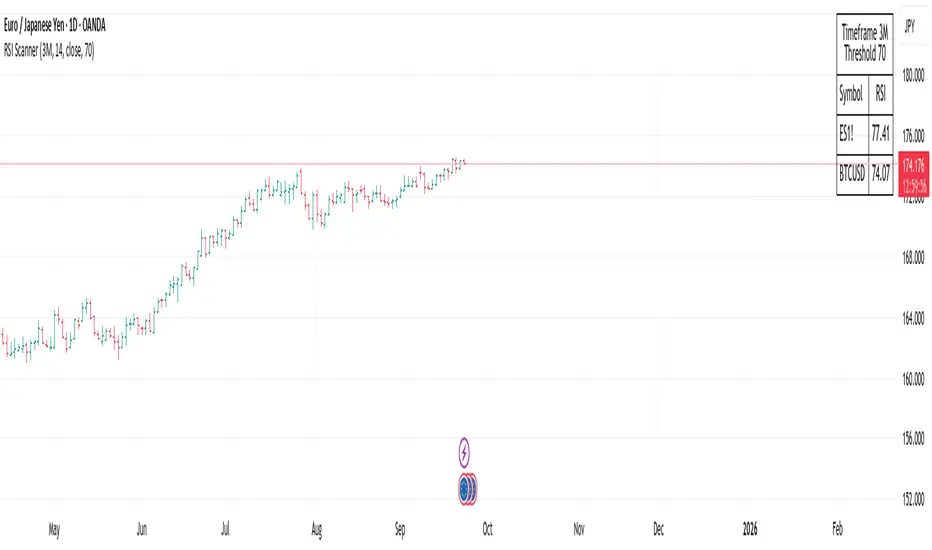
RSI ScannerRSI Scanner
This script scans a custom list of symbols and displays their RSI values for a selected higher timeframe (default: 3M). It provides a quick way to monitor multiple markets in one place without switching charts.
Features:
Customizable timeframe for RSI calculation (default: 3M).
Adjustable RSI length and source input.
Flexible filter: display all symbols or only those with RSI above a chosen threshold.
Input your own list of symbols (stocks, forex, futures, crypto) via a text field.
Results displayed in a clean, table directly on the chart.
Automatic column split when the symbol list is long.
Table header shows selected timeframe and filter settings for clarity.
How to use:
Add the script to your chart.
Open the Inputs panel.
In Symbols List, enter the tickers you want to track, separated by commas (e.g. AAPL, TSLA, EURUSD, BTCUSD).
Set the desired Timeframe (e.g. 3M, 1M, W).
Adjust RSI Length and Source if needed.
Enable or disable filtering:
If filtering is enabled, only symbols with RSI ≥ the threshold will be shown.
If disabled, all entered symbols will be displayed.
The table in the top-right corner will update automatically on the last bar.
Use cases:
Monitor RSI across different asset classes on higher timeframes.
Quickly spot overbought symbols (e.g. RSI > 70) without switching charts.
Create a custom multi-market watchlist tailored to your strategy.
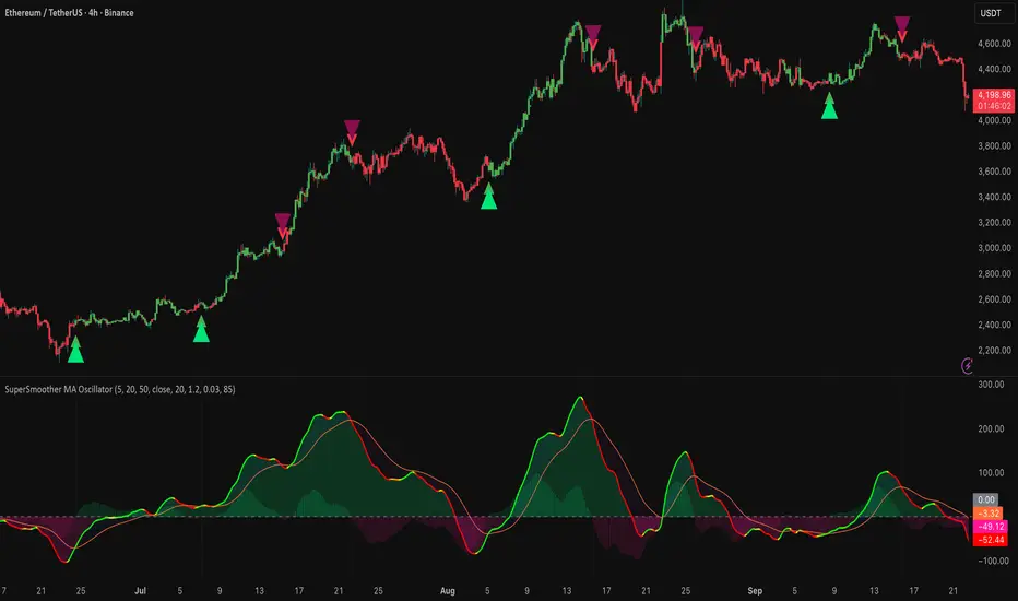
Katz Impact Wave 🚀Overview of the Katz Impact Wave 🚀
The Katz Impact Wave is a momentum oscillator designed to visualize the battle between buyers and sellers. Instead of combining bullish and bearish pressure into a single line, it separates them into two distinct "Impact Waves."
Its primary goal is to generate clear trade signals by identifying when one side gains control, but only when the market has enough volatility to be considered "moving." This built-in filter helps to avoid signals during flat or choppy market conditions.
Indicator Components: Lines & Plots
Impact Waves & Fill
Green Wave (Total Up Impulses): This line represents the cumulative buying pressure. When this line is rising, it indicates that bulls are getting stronger.
Red Wave (Total Down Impulses): This line represents the cumulative selling pressure. When this line is rising, it indicates that bears are getting stronger.
Colored Fill: The shaded area between the two waves provides an at-a-glance view of who is in control.
Lime Fill: Bulls are dominant (Green Wave is above the Red Wave).
Red Fill: Bears are dominant (Red Wave is above the Green Wave).
Background Color
The background color provides crucial context about the market state according to the indicator's logic.
Green Background: The market is in a bullish state (Green Wave is dominant) AND the Rate of Change (ROC) filter confirms the market is actively moving.
Red Background: The market is in a bearish state (Red Wave is dominant) AND the ROC filter confirms the market is actively moving.
Gray Background: The market is considered "not moving" or is in a low-volatility chop. Signals that occur when the background is gray should be viewed with extreme caution or ignored.
Symbols & Pivot Lines
▲ Blue Triangle (Up): This is your long entry signal. It appears on the bar where the Green Wave crosses above the Red Wave while the market is moving.
▼ Orange Triangle (Down): This is your short entry signal. It appears on the bar where the Red Wave crosses above the Green Wave while the market is moving.
Pivot Lines (Solid Green/Red/White Lines): These lines mark confirmed peaks of exhaustion in momentum, not price.
Green Pivot Line: Marks a peak in the Green Wave, signaling buying momentum exhaustion. This can be a warning that the uptrend is losing steam.
Red Pivot Line: Marks a peak in the Red Wave, signaling selling momentum exhaustion. This can be a warning that the downtrend is losing steam.
▼ Yellow Triangle (Compression): This rare signal appears when buying and selling exhaustion pivots happen at the same level. It signifies a point of extreme indecision or equilibrium that often occurs before a major price expansion.
Trading Rules & Strategy
This indicator provides entry signals but does not provide explicit Take Profit or Stop Loss levels. You must use your own risk management rules.
Long Trade Rules
Entry Signal: Wait for a blue ▲ triangle to appear at the top of the indicator panel.
Confirmation: Ensure the background color is green, confirming the market is in a bullish, moving state.
Action: Enter a long (buy) trade at the open of the next candle after the signal appears.
Short Trade Rules
Entry Signal: Wait for an orange ▼ triangle to appear at the bottom of the indicator panel.
Confirmation: Ensure the background color is red, confirming the market is in a bearish, moving state.
Action: Enter a short (sell) trade at the open of the next candle after the signal appears.
Take Profit (TP) & Stop Loss (SL) Ideas
You must develop and test your own exit strategy. Here are some common approaches:
Stop Loss:
Place a stop loss below the most recent significant swing low on the price chart for a long trade, or above the recent swing high for a short trade.
Use an ATR (Average True Range) based stop, such as 2x the ATR value below your entry for a long, to account for market volatility.
Take Profit:
Opposite Signal: The simplest exit is to close your trade when the opposite signal appears (e.g., close a long trade when a short signal ▼ appears).
Momentum Exhaustion: For a long trade, consider taking partial or full profit when a green Pivot Line appears, signaling that buying momentum is peaking.
Fixed Risk/Reward: Use a predetermined risk/reward ratio (e.g., 1:1.5 or 1:2).
Disclaimer
This indicator is a tool for analysis, not a financial advisor or a guaranteed profit system. All trading and investment activities involve substantial risk. You should not risk more than you are prepared to lose. Past performance is not an indication of future results. You are solely responsible for your own trading decisions, risk management, and for backtesting this or any other tool before using it in a live trading environment. This indicator is for educational purposes only.

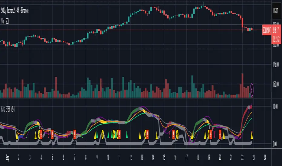
Katz Exploding PowerBand FilterUnderstanding the Katz Exploding PowerBand Filter (EPBF) v2.4
1. Indicator Overview
The Katz Exploding PowerBand Filter (EPBF) is an advanced technical indicator designed to identify moments of expanding bullish or bearish momentum, often referred to as "power." It operates as a standalone oscillator in a separate pane below the main price chart.
Its primary goal is to measure underlying market strength by calculating custom "Bull" and "Bear" power components. These components are then filtered through a versatile moving average and a dual signal line system to generate clear entry and exit signals. This indicator is not a simple momentum oscillator; it uses a unique calculation based on exponential envelopes of both price and squared price to derive its values.
2. On-Chart Lines and Components
The indicator pane consists of five main lines:
Bullish Component (Thick Green/Blue/Yellow/Gray Line): This is the core of the indicator. It represents the calculated bullish "power" or momentum in the market.
Bright Green: Indicates a strong, active long signal condition.
Blue: Shows the bull component is above the MA filter, but the filter itself is still pointing down—a potential sign of a reversal or weakening downtrend.
Yellow: A warning sign that bullish power is weakening and has fallen below the primary signal lines.
Gray: Represents neutral or insignificant bullish power.
Bearish Component (Thick Red/Purple/Yellow/Gray Line): This line represents the calculated bearish "power" or downward momentum.
Bright Red: Indicates a strong, active short signal condition.
Purple: Shows the bear component is above the MA filter, but the filter itself is still pointing down—a sign of potential trend continuation.
Yellow: A warning sign that bearish power is weakening.
Gray: Represents neutral or insignificant bearish power.
MA Filter (Purple Line): This is the main filter, calculated using the moving average type and length you select in the settings (e.g., HullMA, EMA). The Bull and Bear components are compared against this line to determine the underlying trend bias.
Signal Line 1 (Orange Line): A fast Exponential Moving Average (EMA) of the stronger power component. It acts as the first level of dynamic support or resistance for the power lines.
Signal Line 2 (Lime/Gray Line): A slower EMA that acts as a confirmation filter.
Lime Green: The line turns lime when it is rising and the faster Signal Line 1 is above it, indicating a confirmed bullish trend in momentum.
Gray: Indicates a neutral or bearish momentum trend.
3. On-Chart Symbols and Their Meanings
Various characters are plotted at the bottom of the indicator pane to provide clear, actionable signals.
L (Pre-Long Signal): The first sign of a potential long entry. It appears when the Bullish Component rises and crosses above both signal lines for the first time.
S (Pre-Short Signal): The first sign of a potential short entry. It appears when the Bearish Component rises and crosses above both signal lines for the first time.
▲ (Post-Long Signal): A stronger confirmation for a long entry. It appears with the 'L' signal only if the momentum trend is also confirmed bullish (i.e., the slower Signal Line 2 is lime green).
▼ (Post-Short Signal): A stronger confirmation for a short entry. It appears with the 'S' signal only if the momentum trend is confirmed bullish.
Exit / Take-Profit Symbols:
These symbols appear when a power component crosses below a line, suggesting that momentum is fading and it may be time to take profit.
⚠️ (Exit Signal 1): The Bull/Bear component has crossed below the main MA Filter. This is the first and most sensitive take-profit signal.
☣️ (Exit Signal 2): The Bull/Bear component has crossed below the faster Signal Line 1. This is a moderate take-profit signal.
🚼 (Exit Signal 3): The Bull/Bear component has crossed below the slower Signal Line 2. This is the slowest take-profit signal, suggesting the trend is more definitively exhausted.
4. Trading Strategy and Rules
Long Entry Rules:
Initial Signal: Wait for an L to appear at the bottom of the indicator. This confirms that bullish power is expanding.
Confirmation (Recommended): For a higher-probability trade, wait for a green ▲ symbol to appear. This confirms the underlying momentum trend aligns with the signal.
Entry: Enter a long (buy) position on the opening of the next candle after the signal appears.
Short Entry Rules:
Initial Signal: Wait for an S to appear at the bottom of the indicator. This confirms that bearish power is expanding.
Confirmation (Recommended): For a higher-probability trade, wait for a maroon ▼ symbol to appear. This confirms the underlying momentum trend aligns with the signal.
Entry: Enter a short (sell) position on the opening of the next candle after the signal appears.
Take Profit (TP) Rules:
The indicator provides three levels of take-profit signals. You can choose to exit your entire position or scale out at each level.
For a long trade, exit when you see ⚠️, ☣️, or 🚼 appear below the Bullish Component.
For a short trade, exit when you see ⚠️, ☣️, or 🚼 appear below the Bearish Component.
Stop Loss (SL) Rules:
The indicator does not provide an explicit stop loss. You must use your own risk management rules. Common methods include:
Swing High/Low: For a long position, place your stop loss below the most recent significant swing low on the price chart. For a short position, place it above the most recent swing high.
ATR-Based: Use an Average True Range (ATR) indicator to set a volatility-based stop loss.
Fixed Percentage: Risk a fixed percentage (e.g., 1-2%) of your account on the trade.
5. Disclaimer
This indicator is a tool for technical analysis and should not be considered financial advice. All trading involves significant risk, and past performance is not indicative of future results. The signals generated by this indicator are probabilistic and can result in losing trades. Always use proper risk management, such as setting a stop loss, and never risk more than you are willing to lose. It is recommended to backtest this indicator and use it in conjunction with other forms of analysis before trading with real capital. The indicator should only be used for educational purposes.
Stochastic ExcessThe stochastic indicator is a technical analysis tool used in finance to assess the momentum of an asset’s price. It measures the current closing price relative to its price range over a specified period, usually a short one. This indicator helps identify overbought or oversold conditions, signaling when an asset might be about to reverse its trend.

RSI (1 y 5m) + divergences y rsiNDX 1mWith this indicator we incorporate
RSI of the selected asset in 1 minute.
RSI of the selected asset in 5 minutes.
RSI of the NASDAQ 100 in 1 minute.
Includes divergences that are drawn at the extremes of the RSI of the symbol in 1 minute.
Objective of the indicator:To use it in scalping (intraday) with assets from the Nasdaq 100 ETF, to compare the behavior of the asset against its base index.

SuperSmoother MA OscillatorSuperSmoother MA Oscillator - Ehlers-Inspired Lag-Minimized Signal Framework
Overview
The SuperSmoother MA Oscillator is a crossover and momentum detection framework built on the pioneering work of John F. Ehlers, who introduced digital signal processing (DSP) concepts into technical analysis. Traditional moving averages such as SMA and EMA are prone to two persistent flaws: excessive lag, which delays recognition of trend shifts, and high-frequency noise, which produces unreliable whipsaw signals. Ehlers’ SuperSmoother filter was designed to specifically address these flaws by creating a low-pass filter with minimal lag and superior noise suppression, inspired by engineering methods used in communications and radar systems.
This oscillator extends Ehlers’ foundation by combining the SuperSmoother filter with multi-length moving average oscillation, ATR-based normalization, and dynamic color coding. The result is a tool that helps traders identify market momentum, detect reliable crossovers earlier than conventional methods, and contextualize volatility and phase shifts without being distracted by transient price noise.
Unlike conventional oscillators, which either oversimplify price structure or overload the chart with reactive signals, the SuperSmoother MA Oscillator is designed to balance responsiveness and stability. By preprocessing price data with the SuperSmoother filter, traders gain a signal framework that is clean, robust, and adaptable across assets and timeframes.
Theoretical Foundation
Traditional MA oscillators such as MACD or dual-EMA systems react to raw or lightly smoothed price inputs. While effective in some conditions, these signals are often distorted by high-frequency oscillations inherent in market data, leading to false crossovers and poor timing. The SuperSmoother approach modifies this dynamic: by attenuating unwanted frequencies, it preserves structural price movements while eliminating meaningless noise.
This is particularly useful for traders who need to distinguish between genuine market cycles and random short-term price flickers. In practical terms, the oscillator helps identify:
Early trend continuations (when fast averages break cleanly above/below slower averages).
Preemptive breakout setups (when compressed oscillator ranges expand).
Exhaustion phases (when oscillator swings flatten despite continued price movement).
Its multi-purpose design allows traders to apply it flexibly across scalping, day trading, swing setups, and longer-term trend positioning, without needing separate tools for each.
The oscillator’s visual system - fast/slow lines, dynamic coloration, and zero-line crossovers - is structured to provide trend clarity without hiding nuance. Strong green/red momentum confirms directional conviction, while neutral gray phases emphasize uncertainty or low conviction. This ensures traders can quickly gauge the market state without losing access to subtle structural signals.
How It Works
The SuperSmoother MA Oscillator builds signals through a layered process:
SuperSmoother Filtering (Ehlers’ Method)
At its core lies Ehlers’ two-pole recursive filter, mathematically engineered to suppress high-frequency components while introducing minimal lag. Compared to traditional EMA smoothing, the SuperSmoother achieves better spectral separation - it allows meaningful cyclical market structures to pass through, while eliminating erratic spikes and aliasing. This makes it a superior preprocessing stage for oscillator inputs.
Fast and Slow Line Construction
Within the oscillator framework, the filtered price series is used to build two internal moving averages: a fast line (short-term momentum) and a slow line (longer-term directional bias). These are not plotted directly on the chart - instead, their relationship is transformed into the oscillator values you see.
The interaction between these two internal averages - crossovers, separation, and compression - forms the backbone of trend detection:
Uptrend Signal : Fast MA rises above the slow MA with expanding distance, generating a positive oscillator swing.
Downtrend Signal : Fast MA falls below the slow MA with widening divergence, producing a negative oscillator swing.
Neutral/Transition : Lines compress, flattening the oscillator near zero and often preceding volatility expansion.
This design ensures traders receive the information content of dual-MA crossovers while keeping the chart visually clean and focused on the oscillator’s dynamics.
ATR-Based Normalization
Markets vary in volatility. To ensure the oscillator behaves consistently across assets, ATR (Average True Range) normalization scales outputs relative to prevailing volatility conditions. This prevents the oscillator from appearing overly sensitive in calm markets or too flat during high-volatility regimes.
Dynamic Color Coding
Color transitions reflect underlying market states:
Strong Green : Bullish alignment, momentum expanding.
Strong Red : Bearish alignment, momentum expanding.
These visual cues allow traders to quickly gauge trend direction and strength at a glance, with expanding colors indicating increasing conviction in the underlying momentum.
Interpretation
The oscillator offers a multi-dimensional view of price dynamics:
Trend Analysis : Fast/slow line alignment and zero-line interactions reveal trend direction and strength. Expansions indicate momentum building; contractions flag weakening conditions or potential reversals.
Momentum & Volatility : Rapid divergence between lines reflects increasing momentum. Compression highlights periods of reduced volatility and possible upcoming expansion.
Cycle Awareness : Because of Ehlers’ DSP foundation, the oscillator captures market cycles more cleanly than conventional MA systems, allowing traders to anticipate turning points before raw price action confirms them.
Divergence Detection : When oscillator momentum fades while price continues in the same direction, it signals exhaustion - a cue to tighten stops or anticipate reversals.
By focusing on filtered, volatility-adjusted signals, traders avoid overreacting to noise while gaining early access to structural changes in momentum.
Strategy Integration
The SuperSmoother MA Oscillator adapts across multiple trading approaches:
Trend Following
Enter when fast/slow alignment is strong and expanding:
A fast line crossing above the slow line with expanding green signals confirms bullish continuation.
Use ATR-normalized expansion to filter entries in line with prevailing volatility.
Breakout Trading
Periods of compression often precede breakouts:
A breakout occurs when fast lines diverge decisively from slow lines with renewed green/red strength.
Exhaustion and Reversals
Oscillator divergence signals weakening trends:
Flattening momentum while price continues trending may indicate overextension.
Traders can exit or hedge positions in anticipation of corrective phases.
Multi-Timeframe Confluence
Apply the oscillator on higher timeframes to confirm the directional bias.
Use lower timeframes for refined entries during compression → expansion transitions.
Technical Implementation Details
SuperSmoother Algorithm (Ehlers) : Recursive two-pole filter minimizes lag while removing high-frequency noise.
Oscillator Framework : Fast/slow MAs derived from filtered prices.
ATR Normalization : Ensures consistent amplitude across market regimes.
Dynamic Color Engine : Aligns visual cues with structural states (expansion and contraction).
Multi-Factor Analysis : Combines crossover logic, volatility context, and cycle detection for robust outputs.
This layered approach ensures the oscillator is highly responsive without overloading charts with noise.
Optimal Application Parameters
Asset-Specific Guidance:
Forex : Normalize with moderate ATR scaling; focus on slow-line confirmation.
Equities : Balance responsiveness with smoothing; useful for capturing sector rotations.
Cryptocurrency : Higher ATR multipliers recommended due to volatility.
Futures/Indices : Lower frequency settings highlight structural trends.
Timeframe Optimization:
Scalping (1-5min) : Higher sensitivity, prioritize fast-line signals.
Intraday (15m-1h) : Balance between fast/slow expansions.
Swing (4h-Daily) : Focus on slow-line momentum with fast-line timing.
Position (Daily-Weekly) : Slow lines dominate; fast lines highlight cycle shifts.
Performance Characteristics
High Effectiveness:
Trending environments with moderate-to-high volatility.
Assets with steady liquidity and clear cyclical structures.
Reduced Effectiveness:
Flat/choppy conditions with little directional bias.
Ultra-short timeframes (<1m), where noise dominates.
Integration Guidelines
Confluence : Combine with liquidity zones, order blocks, and volume-based indicators for confirmation.
Risk Management : Place stops beyond slow-line thresholds or ATR-defined zones.
Dynamic Trade Management : Use expansions/contractions to scale position sizes or tighten stops.
Multi-Timeframe Confirmation : Filter lower-timeframe entries with higher-timeframe momentum states.
Disclaimer
The SuperSmoother MA Oscillator is an advanced trend and momentum analysis tool, not a guaranteed profit system. Its effectiveness depends on proper parameter settings per asset and disciplined risk management. Traders should use it as part of a broader technical framework and not in isolation.
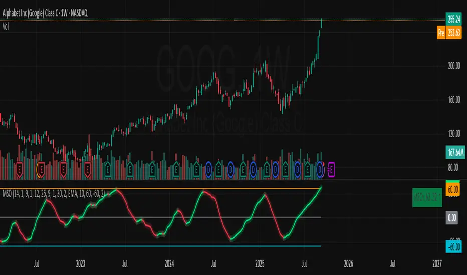
Momentum Shift Oscillator (MSO) [SharpStrat]Momentum Shift Oscillator (MSO)
The Momentum Shift Oscillator (MSO) is a custom-built oscillator that combines the best parts of RSI, ROC, and MACD into one clean, powerful indicator. Its goal is to identify when momentum shifts are happening in the market, filtering out noise that a single momentum tool might miss.
Why MSO?
Most traders rely on just one momentum indicator like RSI, MACD, or ROC. Each has strengths, but also weaknesses:
RSI → great for overbought/oversold, but often lags in strong trends.
ROC (Rate of Change) → captures price velocity, but can be too noisy.
MACD Histogram → shows trend strength shifts, but reacts slowly at times.
By blending all three (with adjustable weights), MSO gives a balanced view of momentum. It captures trend strength, velocity, and exhaustion in one oscillator.
How MSO Works
Inputs:
RSI, ROC, and MACD Histogram are calculated with user-defined lengths.
Each is normalized (so they share the same scale of -100 to +100).
You can set weights for RSI, ROC, and MACD to emphasize different components.
The components are blended into a single oscillator value.
Smoothing (SMA, EMA, or WMA) is applied.
MSO plots as a smooth line, color-coded by slope (green rising, red falling).
Overbought and oversold levels are plotted (default: +60 / -60).
A zero line helps identify bullish vs bearish momentum shifts.
How to trade with MSO
Zero line crossovers → crossing above zero suggests bullish momentum; crossing below zero suggests bearish momentum.
Overbought and oversold zones → values above +60 may indicate exhaustion in bullish moves; values below -60 may signal exhaustion in bearish moves.
Slope of the line → a rising line shows strengthening momentum, while a falling line signals fading momentum.
Divergences → if price makes new highs or lows but MSO does not, it can point to a possible reversal.
Why MSO is Unique
Combines trend + momentum + velocity into one view.
Filters noise better than standalone RSI/MACD.
Adapts to both trend-following and mean-reversion styles.
Can be used across any timeframe for confirmation.

CuteWilly Oscillator_SKThis is a potent combination of Williams % R , EMA & SMA on Williams % R alongwith input from RSI as well. Gives very good picture of the trend, trend reversal and strength of the trend as well.

Mean Reversion Probability Zones [BigBeluga]🔵 OVERVIEW
The Mean Reversion Probability Zones indicator measures the likelihood of price reverting back toward its mean . By analyzing oscillator dynamics (RSI, MFI, or Stochastic), it calculates probability zones both above and below the oscillator. These zones are visualized as histograms, colored regions on the main chart, and a compact dashboard, helping traders spot when the market is statistically stretched and more likely to revert.
🔵 CONCEPTS
Mean Reversion : The tendency of price to return to its average after significant extensions.
Oscillator-Based Analysis : Uses RSI, MFI, or Stochastic as the base signal for detecting overextension.
Probability Model : The probability of reversion is computed using three factors:
Whether the oscillator is rising or declining.
Whether the oscillator is above or below user-defined thresholds.
The oscillator’s actual value (distance from equilibrium).
Dual-Zone Output :
Upper histogram = probability of downward mean reversion.
Lower histogram = probability of upward mean reversion.
Historical Extremes : The dashboard highlights the recent maximum probability values for both upward and downward scenarios.
🔵 FEATURES
Oscillator Choice : Switch between RSI, MFI, and Stochastic.
Customizable Zones : User-defined upper/lower thresholds with independent colors.
Probability Histograms :
Above oscillator → down reversion probability.
Below oscillator → up reversion probability.
Colored Gradient Zones on Chart : Visual overlays showing where mean reversion probabilities are strongest.
Probability Labels : Percentages displayed next to histogram values for clarity.
Dashboard : Compact table in the corner showing the recent maximum probabilities for both upward and downward mean reversion.
Overlay Compatibility : Works in both chart pane and sub-pane with oscillators.
🔵 HOW TO USE
Set Oscillator : Choose RSI, MFI, or Stochastic depending on your strategy style.
Adjust Zones : Define upper/lower bounds for when oscillator values indicate strong overbought/oversold conditions.
Interpret Histograms :
Orange (upper) histogram → higher chance of a pullback/downward mean reversion.
Green (lower) histogram → higher chance of upward reversion/bounce.
Watch Gradient Zones : On the main chart, shaded areas highlight where probability of mean reversion is elevated.
Consult Dashboard : Use the “Recent MAX” values to understand how strong recent reversion probabilities have been in either direction.
Confluence Strategy : Combine with support/resistance, order flow, or trend filters to avoid counter-trend trades.
🔵 CONCLUSION
The Mean Reversion Probability Zones provides traders with an advanced way to quantify and visualize mean reversion opportunities. By blending oscillator momentum, threshold logic, and probability calculations, it highlights when markets are statistically stretched and primed for reversal. Whether you are a contrarian trader or simply looking for exhaustion signals to fade, this tool helps bring structure and clarity to mean reversion setups.

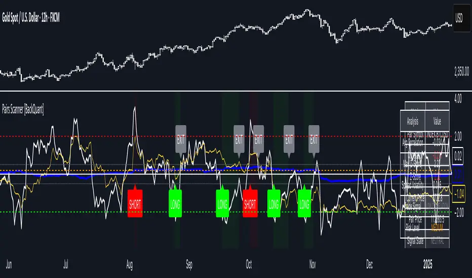
Pairs Trading Scanner [BackQuant]Pairs Trading Scanner
What it is
This scanner analyzes the relationship between your chart symbol and a chosen pair symbol in real time. It builds a normalized “spread” between them, tracks how tightly they move together (correlation), converts the spread into a Z-Score (how far from typical it is), and then prints clear LONG / SHORT / EXIT prompts plus an at-a-glance dashboard with the numbers that matter.
Why pairs at all?
Markets co-move. When two assets are statistically related, their relationship (the spread) tends to oscillate around a mean.
Pairs trading doesn’t require calling overall market direction you trade the relative mispricing between two instruments.
This scanner gives you a robust, visual way to find those dislocations, size their significance, and structure the trade.
How it works (plain English)
Step 1 Pick a partner: Select the Pair Symbol to compare against your chart symbol. The tool fetches synchronized prices for both.
Step 2 Build a spread: Choose a Spread Method that defines “relative value” (e.g., Log Spread, Price Ratio, Return Difference, Price Difference). Each lens highlights a different flavor of divergence.
Step 3 Validate relationship: A rolling Correlation checks if the pair is moving together enough to be tradable. If correlation is weak, the scanner stands down.
Step 4 Standardize & score: The spread is normalized (mean & variability over a lookback) to form a Z-Score . Large absolute Z means “stretched,” small means “near fair.”
Step 5 Signals: When the Z-Score crosses user-defined thresholds with sufficient correlation , entries print:
LONG = long chart symbol / short pair symbol,
SHORT = short chart symbol / long pair symbol,
EXIT = mean reversion into the exit zone or correlation failure.
Core concepts (the three pillars)
Spread Method Your definition of “distance” between the two series.
Guidance:
Log Spread: Focuses on proportional differences; robust when prices live on different scales.
Price Ratio: Classic relative value; good when you care about “X per Y.”
Return Difference: Emphasizes recent performance gaps; nimble for momentum-to-mean plays.
Price Difference: Straight subtraction; intuitive for similar-scale assets (e.g., two ETFs).
Correlation A rolling score of co-movement. The scanner requires it to be above your Min Correlation before acting, so you’re not trading random divergence.
Z-Score “How abnormal is today’s spread?” Positive = chart richer than pair; negative = cheaper. Thresholds define entries/exits with transparent, statistical context.
What you’ll see on the chart
Correlation plot (blue line) with a dashed Min Correlation guide. Above the line = green zone for signals; below = hands off.
Z-Score plot (white line) with colored, dashed Entry bands and dotted Exit bands. Zero line for mean.
Normalized spread (yellow) for a quick “shape read” of recent divergence swings.
Signal markers :
LONG (green label) when Z < –Entry and corr OK,
SHORT (red label) when Z > +Entry and corr OK,
EXIT (gray label) when Z returns inside the Exit band or correlation drops below the floor.
Background tint for active state (faint green for long-spread stance, faint red for short-spread stance).
The two built-in dashboards
Statistics Table (top-right)
Pair Symbol Your chosen partner.
Correlation Live value vs. your minimum.
Z-Score How stretched the spread is now.
Current / Pair Prices Real-time anchors.
Signal State NEUTRAL / LONG / SHORT.
Price Ratio Context for ratio-style setups.
Analysis Table (bottom-right)
Avg Correlation Typical co-movement level over your window.
Max |Z| The recent extremes of dislocation.
Spread Volatility How “lively” the spread has been.
Trade Signal A human-readable prompt (e.g., “LONG A / SHORT B” or “NO TRADE” / “LOW CORRELATION”).
Risk Level LOW / MEDIUM / HIGH based on current stretch (absolute Z).
Signals logic (plain English)
Entry (LONG): The spread is unusually negative (chart cheaper vs pair) and correlation is healthy. Expect mean reversion upward in the spread: long chart, short pair.
Entry (SHORT): The spread is unusually positive (chart richer vs pair) and correlation is healthy. Expect mean reversion downward in the spread: short chart, long pair.
Exit: The spread relaxes back toward normal (inside your exit band), or correlation deteriorates (relationship no longer trusted).
A quick, repeatable workflow
1) Choose your pair in context (same sector/theme or known macro link). Think: “Do these two plausibly co-move?”
2) Pick a spread lens that matches your narrative (ratio for relative value, returns for short-term performance gaps, etc.).
3) Confirm correlation is above your floor no corr, no trade.
4) Wait for a stretch (Z beyond Entry band) and a printed LONG / SHORT .
5) Manage to the mean (EXIT band) or correlation failure; let the scanners’ state/labels keep you honest.
Settings that matter (and why)
Spread Method Defines the “mispricing” you care about.
Correlation Period Longer = steadier regime read, shorter = snappier to regime change.
Z-Score Period The window that defines “normal” for the spread; it sets the yardstick.
Use Percentage Returns Normalizes series when using return-based logic; keep on for mixed-scale assets.
Entry / Exit Thresholds Set your stretch and your target reversion zone. Wider entries = rarer but stronger signals.
Minimum Correlation The gatekeeper. Raising it favors quality over quantity.
Choosing pairs (practical cheat sheet)
Same family: two index ETFs, two oil-linked names, two gold miners, two L1 tokens.
Hedge & proxy: stock vs. sector ETF, BTC vs. BTC index, WTI vs. energy ETF.
Cross-venue or cross-listing: instruments that are functionally the same exposure but price differently intraday.
Reading the cues like a pro
Divergence shape: The yellow normalized spread helps you see rhythm fast spike and snap-back versus slow grind.
Corr-first discipline: Don’t fight the “Min Correlation” line. Good pairs trading starts with a relationship you can trust.
Exit humility: When Z re-centers, let the EXIT do its job. The edge is the journey to the mean, not overstaying it.
Frequently asked (quick answers)
“Long/Short means what exactly?”
LONG = long the chart symbol and short the pair symbol.
SHORT = short the chart symbol and long the pair symbol.
“Do I need same price scales?” No. The spread methods normalize in different ways; choose the one that fits your use case (log/ratio are great for mixed scales).
“What if correlation falls mid-trade?” The scanner will neutralize the state and print EXIT . Relationship first; trade second.
Field notes & patterns
Snap-back days: After a one-sided session, return-difference spreads often flag cleaner intraday mean reversions.
Macro rotations: Ratio spreads shine during sector re-weights (e.g., value vs. growth ETFs); look for steady corr + elevated |Z|.
Event bleed-through: If one symbol reacts to news and its partner lags, Z often flags a high-quality, short-horizon re-centering.
Display controls at a glance
Show Statistics Table Live state & key numbers, top-right.
Show Analysis Table Context/risk read, bottom-right.
Show Correlation / Spread / Z-Score Toggle the sub-charts you want visible.
Show Entry/Exit Signals Turn markers on/off as needed.
Coloring Adjust Long/Short/Neutral and correlation line colors to match your theme.
Alerts (ready to route to your workflow)
Pairs Long Entry Z falls through the long threshold with correlation above minimum.
Pairs Short Entry Z rises through the short threshold with correlation above minimum.
Pairs Trade Exit Z returns to neutral or the relationship fails your correlation floor.
Correlation Breakdown Rolling correlation crosses your minimum; relationship caution.
Final notes
The scanner is designed to keep you systematic: require relationship (correlation), quantify dislocation (Z-Score), act when stretched, stand down when it normalizes or the relationship degrades. It’s a full, visual loop for relative-value trading that stays out of your way when it should and gets loud only when the numbers line up.
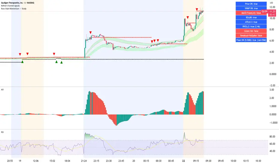
Ross-Style Momentum — StudyRoss-Style Momentum — Study
This indicator is designed to identify high-probability breakout setups inspired by Ross Cameron’s momentum trading style. It combines multiple filters and confirmations to highlight strong long opportunities, while giving traders full control over visibility and thresholds.
Core Features:
Price Range Filter: Only signals when price is between a defined min/max range (ideal for small-cap momentum).
VWAP Alignment: Ensures trades are biased to the long side only when price is above VWAP (optional).
MACD Momentum Check: Requires a fresh MACD bullish crossover within a user-defined lookback.
RSI & ATR Filters: Prevents chasing overextended moves (RSI ceiling) and ignores low-volatility tickers (ATR floor).
Relative Volume (RVOL): Confirms unusual trading activity with minimum RVOL thresholds.
Breakout & Volume Spike: Detects flat-top/base breakouts with volume expansion.
Higher Lows Option: Optional requirement for a constructive higher-lows pattern before breakout.
Float Filter: User-provided float value to avoid large-float stocks if desired.
Visual Tools:
Optional VWAP, Base High/Low, and RVOL plots.
Long setup markers (green labels under qualifying bars).
Background highlight when all conditions align.
Real-time dashboard (top-right) showing pass/fail status of each filter.
Alerts:
Triggers an alert when a full long setup condition is met.
This study does not place trades; it is intended as a signal and confirmation tool for discretionary traders who want to visually validate Ross-style momentum breakout conditions.
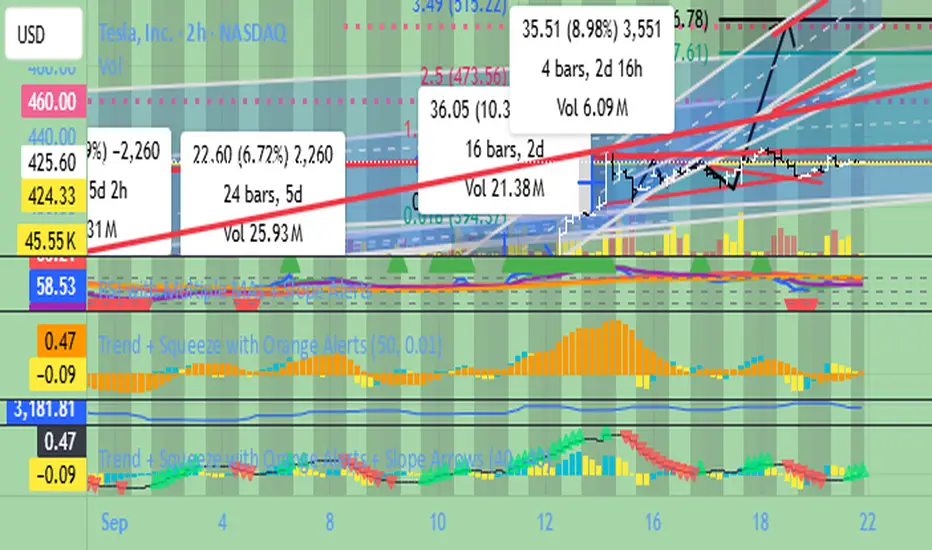
Trend + Squeeze High VolatilityGood for High Volatility Stocks and Options
Trend and Squeeze High Volatility
Good For High Volatility Stocks and Options
Trend + Squeeze with Fast Flexible Transition ESGood for ES.
Trend and Squeeze with Fast Flexible Transition
Good for ES.
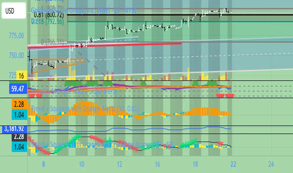
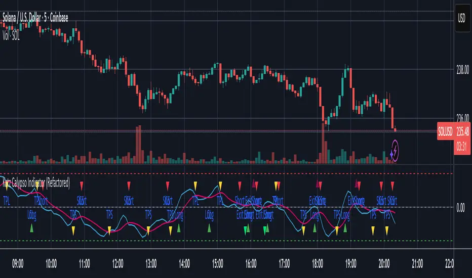
Katz Calypso Indicator (Refactored)Overview
The Katz Calypso Indicator is a comprehensive momentum oscillator designed to identify potential entry and exit points in the market. At its core, it uses the True Strength Index (TSI) to gauge the strength and direction of a trend. To enhance signal accuracy and reduce false positives, the indicator integrates several optional filters, including the Waddah Attar Explosion, an EMA filter, and an ATR filter. It also provides an optional RVGI-based exit signal system.
This tool is designed to provide a clear, visual representation of market momentum, with customizable filters to adapt to various trading styles and market conditions.
How to Use the Indicator
The indicator is displayed in a separate pane below the main price chart.
TSI Line (Blue): This is the main oscillator line. Its position relative to the zero line indicates the overall trend bias (above 0 is bullish, below is bearish).
Signal Line (Red): A moving average of the TSI line. Crossovers between the TSI and Signal Line are the primary triggers for trade signals.
Zero Line: The centerline of the oscillator. A cross of the Zero Line can indicate a significant shift in momentum.
Overbought/Oversold Levels: These user-defined levels (defaulting to 65 and -65) help identify potential exhaustion points in a trend, which can be used for taking profits.
On-Chart Signals: The indicator plots shapes directly on the chart to make signals easy to spot:
Green Triangles (Up): Indicate long entry or continuation signals.
Red Triangles (Down): Indicate short entry or continuation signals.
Yellow Triangles: Suggest taking profits.
Maroon/Lime Triangles: Indicate an exit based on a signal cross (like RVGI or the Zero Line).
Trading Rules
Long Trade Rules
Entry: A long trade is signaled when ALL of the following conditions are met:
The blue TSI Line crosses above the red Signal Line.
The blue TSI Line is above the 0 Zero Line.
All enabled filters (Waddah Attar, EMA, ATR) confirm bullish conditions.
A green triangle labeled "Long" will appear below the price.
Exit (Take Profit): A take-profit signal for a long trade is generated when either of these occurs:
The TSI Line crosses below the Overbought level.
The TSI Line crosses back below the Signal Line while still above zero.
A yellow triangle labeled "TPL" (Take Profit Long) will appear above the price.
Exit (Stop/Reverse): A signal to exit a long trade is generated when either of these occurs:
The TSI Line crosses below the 0 Zero Line.
The RVGI Exit filter is enabled and generates a bearish crossover signal.
A maroon triangle labeled "Exit Long" will appear above the price.
Short Trade Rules
Entry: A short trade is signaled when ALL of the following conditions are met:
The blue TSI Line crosses below the red Signal Line.
The blue TSI Line is below the 0 Zero Line.
All enabled filters (Waddah Attar, EMA, ATR) confirm bearish conditions.
A red triangle labeled "Short" will appear above the price.
Exit (Take Profit): A take-profit signal for a short trade is generated when either of these occurs:
The TSI Line crosses above the Oversold level.
The TSI Line crosses back above the Signal Line while still below zero.
A yellow triangle labeled "TPS" (Take Profit Short) will appear below the price.
Exit (Stop/Reverse): A signal to exit a short trade is generated when either of these occurs:
The TSI Line crosses above the 0 Zero Line.
The RVGI Exit filter is enabled and generates a bullish crossover signal.
A lime green triangle labeled "Exit Short" will appear below the price.
Optional Filters
You can enable or disable these filters in the indicator's settings to fine-tune its sensitivity.
Waddah Attar Explosion Filter: This filter measures trend strength and volatility. When enabled, it ensures that entries are only taken during periods of strong, confirmed momentum, helping to avoid sideways or choppy markets.
EMA Price Filter: A classic trend filter. When enabled, it will only allow long entries if the price is above the specified Exponential Moving Average and short entries only if the price is below it.
ATR Filter: This acts as a volatility-based filter to prevent chasing a move. It helps ensure that you are not entering a long trade when the price has already moved too far above its EMA, or vice-versa for a short trade.
RVGI Exit Filter: The Relative Vigor Index (RVGI) is used here exclusively as an exit signal. When enabled, a crossover of the RVGI and its signal line can provide an earlier exit signal before the TSI crosses the zero line, potentially locking in profits sooner.
Disclaimer: This indicator is provided for educational and informational purposes only. It is not financial advice. Trading carries a high level of risk, and you can lose more than your initial investment. You should use this indicator at your own risk and discretion. Always conduct your own research and consider your risk tolerance before making any trading decisions.
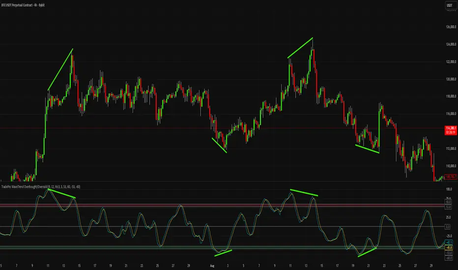
Simplified Wave Trend Overbought/OversoldThis is just a variation of the popular wave trend that I find to be nicer to look at.
BioSwarm Imprinter™BioSwarm Imprinter™ — Agent-Based Consensus for Traders
What it is
BioSwarm Imprinter™ is a non-repainting, agent-based sentiment oscillator. It fuses many short-to-medium lookback “opinions” into one 0–100 consensus line that is easy to read at a glance (50 = neutral, >55 bullish bias, <45 bearish bias). The engine borrows from swarm intelligence: many simple voters (agents) adapt their influence over time based on how well they’ve been predicting price, so the crowd gets smarter as conditions change.
Use it to:
• Detect emerging trends sooner without overreacting to noise.
• Filter mean-reversion vs continuation opportunities.
• Gate entries with a confidence score that reflects both strength and persistence of the move.
• Combine with your execution tools (VWAP/ORB/levels) as a state filter rather than a trade signal by itself.
⸻
Why it’s different
• Swarm learning: Each agent improves or decays its “fitness” depending on whether its vote matched the next bar’s direction. High-fitness agents matter more; weak agents fade.
• Multi-horizon by design: The crowd is composed of fixed, simple lookbacks spread from lenMin to lenMax. You get a blended, robust view instead of a single fragile parameter.
• Two complementary lenses: Each agent evaluates RSI-style balance (via Wilder’s RMA) and momentum (EMA deviation). You decide the weight of each.
• No repaint, no MTF pitfalls: Everything runs on the chart’s timeframe with bar-close confirmation; no request.security() or forward references.
• Actionable UI: A clean consensus line, optional regime background, confidence heat, and triangle markers when thresholds are crossed.
⸻
What you see on the chart
• Consensus line (0–100): Smoothed to your preference; color/area makes bull/bear zones obvious.
• Regime coloring (optional): Light green in bull zone, light red in bear zone; neutral otherwise.
• Confidence heat: A small gauge/number (0–100) that combines distance from neutral and recent persistence.
• Markers (optional): Triangles when consensus crosses up through your bull threshold (e.g., 55) or down through your bear threshold (e.g., 45).
• Info panel (optional): Consensus value, regime, confidence, number of agents, and basic diagnostics.
⸻
How it works (under the hood)
1. Horizon bins: The range is divided into numBins. Each bin has a fixed, simple integer length (crucial for Pine’s safety rules).
2. Per-bin features (computed every bar):
• RSI-style balance using Wilder’s RMA (not ta.rsi()), then mapped to −1…+1.
• Momentum as (close − EMA(L)) / EMA(L) (dimensionless drift).
3. Agent vote: For its assigned bin, an agent forms a weighted score: score = wRSI*RSI_like + wMOM*Momentum. A small dead-band near zero suppresses chop; votes are +1/−1/0.
4. Fitness update (bar close): If the agent’s previous vote agreed with the next bar’s direction, multiply its fitness by learnGain; otherwise by learnPain. Fitness is clamped so it never explodes or dies.
5. Consensus: Weighted average of all votes using fitness as weights → map to 0–100 and smooth with EMA.
Why it doesn’t repaint:
• No future references, no MTF resampling, fitness updates only on confirmed bars.
• All TA primitives (RMA/EMA/deltas) are computed every bar unconditionally.
⸻
Signals & confidence
• Bullish bias: consensus ≥ bullThr (e.g., 55).
• Bearish bias: consensus ≤ bearThr (e.g., 45).
• Confidence (0–100):
• Distance score: how far consensus is from 50.
• Momentum score: how strong the recent change is versus its recent average.
• Combined into a single gate; start filtering entries at ≥60 for higher quality.
Tip: For range sessions, raise thresholds (60/40) and increase smoothing; for momentum sessions, lower smoothing and keep thresholds at 55/45.
⸻
Inputs you’ll actually tune
• Agents & horizons:
• N_agents (e.g., 64–128)
• lenMin / lenMax (e.g., 6–30 intraday, 10–60 swing)
• numBins (e.g., 12–24)
• Weights & smoothing:
• wRSI vs wMOM (e.g., 0.7/0.3 for FX & indices; 0.6/0.4 for crypto)
• deadBand (0.03–0.08)
• consSmooth (3–8)
• Thresholds & hygiene:
• bullThr/bearThr (55/45 default)
• cooldownBars to avoid signal spam
⸻
Playbooks (ready-to-use)
1) Breakout / Trend continuation
• Timeframe: 15m–1h for day/swing.
• Filter: Take longs only when consensus > 55 and confidence ≥ 60.
• Execution: Use your ORB/VWAP/pullback trigger for entry. Trail with swing lows or 1.5×ATR. Exit on a close back under 50 or when a bearish signal prints.
2) Mean reversion (fade)
• When: Sideways days or low-volatility clusters.
• Setup: Increase deadBand and consSmooth.
• Signal: Bearish fades when consensus rolls over below ≈55 but stays above 50; bullish fades when it rolls up above ≈45 but stays below 50.
• Targets: The neutral zone (~50) as the first take-profit.
3) Multi-TF alignment
• Keep BioSwarm on 1H for bias, execute on 5–15m:
• Only take entries in the direction of the 1H consensus.
• Skip counter-bias scalps unless confidence is very low (explicit mean-reversion plan).
⸻
Integrations that work
• DynamoSent Pro+ (macro bias): Only act when macro bias and swarm consensus agree.
• ORB + Session VWAP Pro: Trade London/NY ORB breakouts that retest while consensus >55 (long) or <45 (short).
• Levels/Orderflow: BioSwarm is your “go / no-go”; execution stays with your usual triggers.
⸻
Quick start
1. Drop the indicator on a 1H chart.
2. Start with: N_agents=64, lenMin=6, lenMax=30, numBins=16, deadBand=0.06, consSmooth=5, thresholds 55/45.
3. Trade only when confidence ≥ 60.
4. Add your favorite execution tool (VWAP/levels/OR) for entries & exits.
⸻
Non-repainting & safety notes
• No request.security(); no hidden lookahead.
• Bar-close confirmation for fitness and signals.
• All TA calls are unconditional (no “sometimes called” warnings).
• No series-length inputs to RSI/EMA — we use RMA/EMA formulas that accept fixed simple ints per bin.
⸻
Known limits & tips
• Too many signals? Raise deadBand, increase consSmooth, widen thresholds to 60/40.
• Too few signals? Lower deadBand, reduce consSmooth, narrow thresholds to 53/47.
• Over-fitting risk: Keep learnGain/learnPain modest (e.g., ×1.04 / ×0.96).
• Compute load: Large N_agents × numBins is heavier; scale to your device.
⸻
Example recipes
EURUSD 1H (swing):
lenMin=8, lenMax=34, numBins=16, wRSI=0.7, wMOM=0.3, deadBand=0.06, consSmooth=6, thr=55/45
Buy breakouts when consensus >55 and confidence ≥60; confirm with 5–15m pullback to VWAP or level.
SPY 15m (US session):
lenMin=6, lenMax=24, numBins=12, consSmooth=4, deadBand=0.05
On trend days, stay with longs as long as consensus >55; add on shallow pullbacks.
BTC 1H (24/7):
Increase momentum weight: wRSI=0.6, wMOM=0.4, extend lenMax to ~50. Use dynamic stops (ATR) and partials on strong verticals.
⸻
Final word
BioSwarm is a state engine: it tells you when the market is primed to continue or mean-revert. Pair it with your entries and risk framework to turn that state into trades. If you’d like, I can supply a companion strategy template that consumes the consensus and back-tests the three playbooks (Breakout/Fade/Flip) with standard risk management.

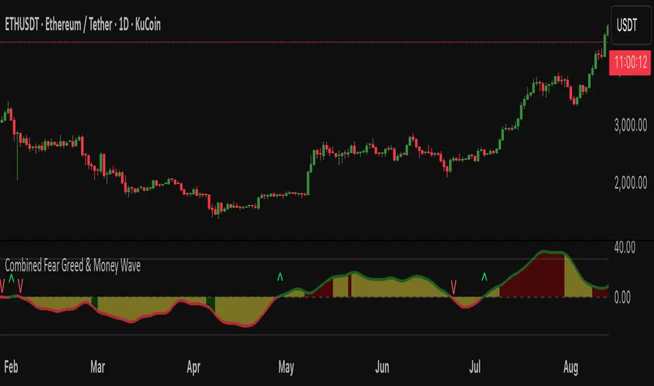
Fear Greed zones and Money Waves FusedThis indicator, named "Fear Greed zones and Money Waves" combines a smoothed Money Flow Index (MFI)-based wave and the Relative Strength Index (RSI) to visualize market sentiment through fear and greed zones and generate buy/sell signals.
Core Functions
- It calculates a zero-centered and smoothed version of the MFI (MoneyWave) using configurable smoothing methods (SMA, EMA, RMA) with parameters for length and smoothing intensity.
- It uses RSI to define fear and greed zones based on user-defined thresholds (e.g., RSI below 30 indicates fear, above 70 indicates greed).
- The MoneyWave area is color-coded based on these fear/greed RSI zones: dark green for fear, dark red for greed, and yellow neutral.
- The edge line of the MoneyWave shows bullish (lime) when above zero and bearish (red) when below zero.
Visual Elements
- Plots the MoneyWave as a colored area with an edge line.
- Displays horizontal lines representing the zero line and upper/lower bounds derived from MFI thresholds.
- Optionally shows direction change arrows when the MoneyWave sign changes and labels indicating BUY or SELL signals based on MoneyWave crossing zero combined with fear/greed conditions.
Trading Signals and Alerts
- Buy signal triggers when MoneyWave crosses upward through zero while in the fear zone (RSI low).
- Sell signal triggers when MoneyWave crosses downward through zero while in the greed zone (RSI high).
- Alerts can be generated for these buy/sell events.
In summary, this indicator provides a combined measure of money flow momentum (MoneyWave) with market sentiment zones (fear and greed from RSI), helping identify potential market entry and exit points with visual markers and alerts .
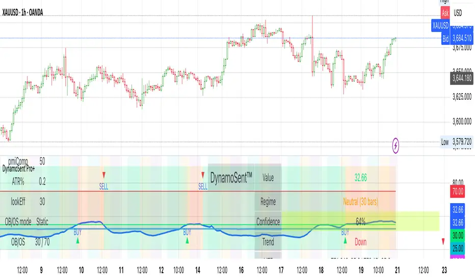
DynamoSent DynamoSent Pro+ — Professional Listing (Preview)
— Adaptive Macro Sentiment (v6)
— Export, Adaptive Lookback, Confidence, Boxes, Heatmap + Dynamic OB/OS
Preview / Experimental build. I’m actively refining this tool—your feedback is gold.
If you spot edge cases, want new presets, or have market-specific ideas, please comment or DM me on TradingView.
⸻
What it is
DynamoSent Pro+ is an adaptive, non-repainting macro sentiment engine that compresses VIX, DXY and a price-based activity proxy (e.g., SPX/sector ETF/your symbol) into a 0–100 sentiment line. It scales context by volatility (ATR%) and can self-calibrate with rolling quantile OB/OS. On top of that, it adds confidence scoring, a plain-English Context Coach, MTF agreement, exportable sentiment for other indicators, and a clean Light/Dark UI.
Why it’s different
• Adaptive lookback tracks regime changes: when volatility rises, we lengthen context; when it falls, we shorten—less whipsaw, more relevance.
• Dynamic OB/OS (quantiles) self-calibrates to each instrument’s distribution—no arbitrary 30/70 lines.
• MTF agreement + Confidence gate reduce false positives by highlighting alignment across timeframes.
• Exportable output: hidden plot “DynamoSent Export” can be selected as input.source in your other Pine scripts.
• Non-repainting rigor: all request.security() calls use lookahead_off + gaps_on; signals wait for bar close.
Key visuals
• Sentiment line (0–100), OB/OS zones (static or dynamic), optional TF1/TF2 overlays.
• Regime boxes (Overbought / Oversold / Neutral) that update live without repaint.
• Info Panel with confidence heat, regime, trend arrow, MTF readout, and Coach sentence.
• Session heat (Asia/EU/US) to match intraday behavior.
• Light/Dark theme switch in Inputs (auto-contrasted labels & headers).
⸻
How to use (examples & recipes)
1) EURUSD (swing / intraday blend)
• Preset: EURUSD 1H Swing
• Chart: 1H; TF1=1H, TF2=4H (default).
• Proxies: Defaults work (VIX=D, DXY=60, Proxy=D).
• Dynamic OB/OS: ON at 20/80; Confidence ≥ 55–60.
• Playbook:
• When sentiment crosses above 50 + margin with Δ ≥ signalK and MTF agreement ≥ 0.5, treat as trend breakout.
• In Oversold with rising Coach & TF agreement, take fade longs back toward mid-range.
• Alerts: Enable Breakout Long/Short and Fade; keep cooldown 8–12 bars.
2) SPY (daytrading)
• Preset: SPY 15m Daytrade; Chart: 15m.
• VIX (D) matters more; preset weights already favor it.
• Start with static 30/70; later try dynamic 25/75 for adaptive thresholds.
• Use Coach: in US session, when it says “Overbought + MTF agree → sell rallies / chase breakouts”, lean momentum-continuation after pullbacks.
3) BTCUSD (crypto, 24/7)
• Preset: BTCUSD 1H; Chart: 1H.
• DXY and BTC.D inform macro tone; keep Carry-forward ON to bridge sparse ticks.
• Prefer Dynamic OB/OS (15/85) for wider swings.
• Fade signals on weekend chop; Breakout when Confidence > 60 and MTF ≥ 1.0.
4) XAUUSD (gold, macro blend)
• Preset: XAUUSD 4H; Chart: 4H.
• Weights tilt to DXY and US10Y (handled by preset).
• Coach + MTF helps separate trend legs from news pops.
⸻
Best practices
• Theme: Switch Light/Dark in Inputs; the panel adapts contrast automatically.
• Export: In another script → Source → DynamoSent Pro+ → DynamoSent Export. Build your own filters/strategies atop the same sentiment.
• Dynamic vs Static OB/OS:
• Static 30/70: fast, universal baseline.
• Dynamic (quantiles): instrument-aware; use 20/80 (default) or 15/85 for choppy markets.
• Confidence gate: Start at 50–60% to filter noise; raise when you want only A-grade setups.
• Adaptive Lookback: Keep ON. For ultra-liquid indices, you can switch it OFF and set a fixed lookback.
⸻
Non-repainting & safety notes
• All request.security() calls use lookahead=barmerge.lookahead_off and gaps=barmerge.gaps_on.
• No forward references; signals & regime flips are confirmed on bar close.
• History-dependent funcs (ta.change, ta.percentile_linear_interpolation, etc.) are computed each bar (not conditionally).
• Adaptive lookback is clamped ≥ 1 to avoid lowest/highest errors.
• Missing-data warning triggers only when all proxies are NA for a streak; carry-forward can bridge small gaps without repaint.
⸻
Known limits & tips
• If a proxy symbol isn’t available on your plan/exchange, you’ll see the NA warning: choose a different symbol via Symbol Search, or keep Carry-forward ON (it defaults to neutral where needed).
• Intraday VIX is sparse—using Daily is intentional.
• Dynamic OB/OS needs enough history (see dynLenFloor). On short histories it gracefully falls back to static levels.
Thanks for trying the preview. Your comments drive the roadmap—presets, new proxies, extra alerts, and integrations.
ARO Pro — Adaptive Regime OscillatorARO Pro — Adaptive Regime Oscillator (v6)
ARO Pro turns your chart into a context-aware decision system. It classifies every bar as Trending (up or down) or Ranging in real time, then switches its math to match the regime: trend strength is measured with an ATR-normalized EMA spread, while range behavior is tracked with a center-based RSI oscillator. The result is cleaner entries, fewer false signals, and faster reads on regime shifts—without repainting.
⸻
How it works (under the hood)
1. Regime Detection (Kaufman ER):
ARO computes Kaufman’s Efficiency Ratio (ER) over a user-defined length.
- ER > threshold → Trending (direction from EMA fast vs. EMA slow)
- ER ≤ threshold → Ranging
2. Adaptive Oscillator Core:
- Trend mode: (EMA(fast) − EMA(slow)) / ATR * 100 → momentum normalized by volatility.
- Range mode: RSI(length) − 50 → mean-reversion pressure around zero.
3. Volatility Filter (optional):
Blocks signals if ATR as % of price is below a floor you set. This reduces noise in thin or quiet markets.
4. MTF Trend Filter (optional & non-repainting):
Confirms signals only if a higher timeframe EMA(fast) > EMA(slow) for longs (or < for shorts). Implemented with lookahead_off and gaps_on.
5. Confirmation & Alerts:
Signals are locked only on bar close (barstate.isconfirmed) and offered via three alert types: ARO Long, ARO Short, ARO Regime Shift.
⸻
What you see on the chart
• Background heat:
• Green = Trending Up, Red = Trending Down, Gray = Range.
• ARO line (panel): Adaptive oscillator (trend/value colors).
• Signal markers: ▲ Long / ▼ Short on confirmed bars.
• Guide lines: Upper/Lower thresholds (±K) and zero line.
• Info Panel (table): Regime, ER, ATR %, ARO, HTF status (OK/BLOCK/OFF), and a Confidence light.
• Debug Overlay (optional): Quick view of thresholds and raw conditions for tuning.
⸻
Inputs (quick reference)
• Signals: Fast/Slow EMA, RSI length, ER length & threshold, oscillator smoothing, signal threshold.
• Filters: ATR length, minimum ATR% (volatility floor), toggle for volatility filter.
• Visuals: Background on/off, Info Panel on/off, Debug overlay on/off.
• MTF (safe): Toggle + HTF timeframe (e.g., 240, D, W).
⸻
Interpreting signals
• Long: Trend regime AND fast EMA > slow EMA AND ARO ≥ +threshold (confirmed bar, filters passing).
• Short: Trend regime AND fast EMA < slow EMA AND ARO ≤ −threshold (confirmed bar, filters passing).
• Regime Shift: Alert when ER moves the market from Range → Trend or flips trend direction.
⸻
Practical use cases & examples
1) Intraday momentum alignment (scalps to day trades)
• Timeframes: 5–15m with HTF filter = 4H.
• Flow:
1. Wait for Trend Up background + HTF OK.
2. Enter on ▲ Long when ARO crosses above +threshold.
3. Stops: 1–1.5× ATR(14) below trigger bar or below last micro swing.
4. Exits: Partial at 1× ATR, trail remainder with an ATR stop or when ARO reverts to zero/Regime Shift.
• Why it works: You’re trading with the dominant higher-timeframe structure while avoiding low-volatility fakeouts.
2) Swing trend following (cleaner trend legs)
• Timeframes: 1H–4H with HTF filter = 1D.
• Flow:
1. Only act in Trend background aligned with HTF.
2. Add on subsequent ▲ signals as ARO maintains positive (or negative) territory.
3. Reduce or exit on Regime Shift (Trend → Range or direction flip) or when ARO crosses back through zero.
• Stops/targets: Initial 1.5–2× ATR; move to breakeven once the trade gains 1× ATR; trail with a multiple-ATR or structure lows/highs.
3) Range tactics (fade the extremes)
• Timeframes: 15m–1H or 1D on mean-reverting names.
• Flow:
1. Act only when background = Range.
2. Fade moves when ARO swings from ±extremes back toward zero near well-defined S/R.
3. Exit at the opposite band or zero line; abort if a Regime Shift to Trend occurs.
• Tip: Increase ER threshold (e.g., 0.35–0.40) to label more bars as Range on choppy instruments.
4) Event days & macro filters
• Approach: Raise the volatility floor (Min ATR%) on macro days (FOMC, CPI).
• Effect: You’ll ignore “fake” micro swings in the minutes leading up to releases and catch only post-event confirmed momentum.
⸻
Parameter tuning guide
• ER Threshold:
• Lower (0.20–0.30) = more Trend bars, more signals, higher noise.
• Higher (0.35–0.45) = stricter trend confirmation, fewer but cleaner signals.
• Signal Threshold (±K):
• Raise to reduce whipsaws; lower for earlier but noisier triggers.
• Volatility Floor (ATR%):
• Thin/quiet assets benefit from a higher floor (e.g., 0.3–0.6).
• Highly liquid futures/forex can work with lower floors.
• HTF Filter:
• Keep it ON when you want higher win consistency; turn OFF for tactical counter-trend plays.
⸻
Alerts (recommended setup)
• “ARO Long” / “ARO Short”: Entry-style alerts on confirmed signals.
• “ARO Regime Shift”: Context alert to scale in/out or switch playbooks (trend vs. range).
All alerts are non-repainting and fire only when the bar closes.
⸻
Best practices & combinations
• Price action & S/R: Use ARO to define when to engage, and price structure to define where (breakout levels, pullback zones).
• VWAP/Session tools: In intraday trends, ▲ signals above VWAP tend to carry; avoid shorts below session VWAP in strong downtrends.
• Risk first: Size by ATR; never let a single ARO event override your max risk per trade.
• Portfolio filter: On indices/ETFs, enable HTF filter and a stricter ER threshold to ride regime legs.
⸻
Non-repaint and implementation notes
• The script does not repaint:
• Signals are computed and locked on bar close (barstate.isconfirmed).
• All higher-timeframe data uses request.security(..., lookahead_off, gaps_on).
• No future indexing or negative offsets are used.
• The Info Panel and Debug overlay are purely visual aids and do not change signal logic.
⸻
Limitations & tips
• Chop sensitivity: In hyper-choppy symbols, consider raising ER threshold and the signal threshold, and enable HTF filter.
• Instrument personality: EMAs/RSI lengths and volatility floor often need a quick 2–3 minute tune per asset class (FX vs. crypto vs. equities).
• No guarantees: ARO improves context and timing, but it is not a promise of profitability—always combine with risk management.
⸻
Quick start (TL;DR)
1. Timeframes: 5–15m intraday (HTF = 4H); 1H–4H swing (HTF = 1D).
2. Use defaults, then tune ER threshold (0.25–0.40) and Signal threshold (±20).
3. Enable Volatility Floor (e.g., 0.2–0.5 ATR%) on quiet assets.
4. Trade ▲ / ▼ only in matching Trend background; fade extremes only in Range background.
5. Set alerts for Long, Short, and Regime Shift; manage risk with ATR stops.
⸻
Author’s note: ARO Pro is designed to be clear, adaptive, and operational out of the box. If you publish variants (e.g., different ER logic, alternative trend cores), please credit the original and document any changes so users can compare behavior reliably.

Synthetic Point & Figure on RSIHere is a detailed description and user guide for the Synthetic Point & Figure RSI indicator, including how to use it for long and short trade considerations:
*
## Synthetic Point & Figure RSI Indicator – User Guide
### What It Is
This indicator applies classic Point & Figure (P&F) charting logic to the Relative Strength Index (RSI) instead of price. It transforms the RSI into synthetic “P&F candles” that filter out noise and highlight significant momentum moves and reversals based on configurable box size and reversal settings.
### How It Works
- The RSI is calculated normally over the selected length.
- The P&F engine tracks movements in the RSI above or below a defined “box size,” creating columns that switch direction only after a larger reversal.
- The synthetic candles connect these filtered RSI values visually, reducing false noise and emphasizing strong RSI trends.
- Optional EMA and SMA overlays on the synthetic P&F RSI allow smoother trend signals.
- Reference RSI levels at 33, 40, 50, 60, and 66 provide further context for momentum strength.
### How to Use for Trading
#### Long (Buy) Considerations
- The synthetic P&F RSI candle direction flips to *up (green candles)* indicating strength in momentum.
- Look for the RSI P&F value moving above the *40 or 50 level*, suggesting increasing bullish momentum.
- Confirmation is stronger if the synthetic RSI is above the EMA or SMA overlays.
- Ideal entries are after a reversal from a synthetic P&F downtrend (red candles) to an uptrend (green candles) near or above these levels.
#### Short (Sell) Considerations
- The candle direction flips to *down (red candles)*, showing weakening momentum or bearish reversal.
- Monitor if the synthetic RSI falls below the *60 or 50 level*, signaling momentum loss.
- Confirm bearish bias if the price is below the EMA or SMA overlays.
- Exit or short positions are signaled when the synthetic candle reverses from green to red near or below these threshold levels.
### Important RSI Levels to Watch
- *Level 33*: Lower bound indicating deep oversold conditions.
- *Level 40*: Early bullish zone suggesting momentum improvement.
- *Level 50*: Neutral midpoint; crossing above often signals bullish strength, below signals weakness.
- *Level 60*: Advanced bullish momentum; breaking below signals potential reversal.
- *Level 66*: Strong overbought area warning of possible pullback.
### Tips
- Use in conjunction with price action analysis and other volume/trend indicators for higher conviction.
- Adjust box size and reversal settings based on instrument volatility and timeframe for ideal filtering.
- The P&F RSI is best for identifying sustained momentum trends and avoiding false RSI whipsaws.
- Combine this indicator’s signals with stop-loss and risk management strategies.
*
This indicator converts RSI momentum analysis into a simplified, noise-filtered P&F chart format, helping traders better visualize and trade momentum shifts. It is especially useful when RSI signal noise can cause confusion in volatile markets.
Let me know if you want me to generate a shorter summary or code alerts based on these levels!
Sources
Relative Strength Index (RSI) — Indicators and Strategies in.tradingview.com
Indicators and strategies in.tradingview.com
Relative Strength Index (RSI) Indicator: Tutorial www.youtube.com
Stochastic RSI (STOCH RSI) in.tradingview.com
RSI Strategy docs.algotest.in
Stochastic RSI Indicator: Tutorial www.youtube.com
Relative Strength Index (RSI): What It Is, How It Works, and ... www.investopedia.com
rsi — Indicators and Strategies in.tradingview.com
Relative Strength Index (RSI) in.tradingview.com
Relative Strength Index (RSI) — Indicators and Strategies www.tradingview.com