TASC 2025.06 Cybernetic Oscillator█ OVERVIEW
This script implements the Cybernetic Oscillator introduced by John F. Ehlers in his article "The Cybernetic Oscillator For More Flexibility, Making A Better Oscillator" from the June 2025 edition of the TASC Traders' Tips . It cascades two-pole highpass and lowpass filters, then scales the result by its root mean square (RMS) to create a flexible normalized oscillator that responds to a customizable frequency range for different trading styles.
█ CONCEPTS
Oscillators are indicators widely used by technical traders. These indicators swing above and below a center value, emphasizing cyclic movements within a frequency range. In his article, Ehlers explains that all oscillators share a common characteristic: their calculations involve computing differences . The reliance on differences is what causes these indicators to oscillate about a central point.
The difference between two data points in a series acts as a highpass filter — it allows high frequencies (short wavelengths) to pass through while significantly attenuating low frequencies (long wavelengths). Ehlers demonstrates that a simple difference calculation attenuates lower-frequency cycles at a rate of 6 dB per octave. However, the difference also significantly amplifies cycles near the shortest observable wavelength, making the result appear noisier than the original series. To mitigate the effects of noise in a differenced series, oscillators typically smooth the series with a lowpass filter, such as a moving average.
Ehlers highlights an underlying issue with smoothing differenced data to create oscillators. He postulates that market data statistically follows a pink spectrum , where the amplitudes of cyclic components in the data are approximately directly proportional to the underlying periods. Specifically, he suggests that cyclic amplitude increases by 6 dB per octave of wavelength.
Because some conventional oscillators, such as RSI, use differencing calculations that attenuate cycles by only 6 dB per octave, and market cycles increase in amplitude by 6 dB per octave, such calculations do not have a tangible net effect on larger wavelengths in the analyzed data. The influence of larger wavelengths can be especially problematic when using these oscillators for mean reversion or swing signals. For instance, an expected reversion to the mean might be erroneous because oscillator's mean might significantly deviate from its center over time.
To address the issues with conventional oscillator responses, Ehlers created a new indicator dubbed the Cybernetic Oscillator. It uses a simple combination of highpass and lowpass filters to emphasize a specific range of frequencies in the market data, then normalizes the result based on RMS. The process is as follows:
Apply a two-pole highpass filter to the data. This filter's critical period defines the longest wavelength in the oscillator's passband.
Apply a two-pole SuperSmoother (lowpass filter) to the highpass-filtered data. This filter's critical period defines the shortest wavelength in the passband.
Scale the resulting waveform by its RMS. If the filtered waveform follows a normal distribution, the scaled result represents amplitude in standard deviations.
The oscillator's two-pole filters attenuate cycles outside the desired frequency range by 12 dB per octave. This rate outweighs the apparent rate of amplitude increase for successively longer market cycles (6 dB per octave). Therefore, the Cybernetic Oscillator provides a more robust isolation of cyclic content than conventional oscillators. Best of all, traders can set the periods of the highpass and lowpass filters separately, enabling fine-tuning of the frequency range for different trading styles.
█ USAGE
The "Highpass period" input in the "Settings/Inputs" tab specifies the longest wavelength in the oscillator's passband, and the "Lowpass period" input defines the shortest wavelength. The oscillator becomes more responsive to rapid movements with a smaller lowpass period. Conversely, it becomes more sensitive to trends with a larger highpass period. Ehlers recommends setting the smallest period to a value above 8 to avoid aliasing. The highpass period must not be smaller than the lowpass period. Otherwise, it causes a runtime error.
The "RMS length" input determines the number of bars in the RMS calculation that the indicator uses to normalize the filtered result.
This indicator also features two distinct display styles, which users can toggle with the "Display style" input. With the "Trend" style enabled, the indicator plots the oscillator with one of two colors based on whether its value is above or below zero. With the "Threshold" style enabled, it plots the oscillator as a gray line and highlights overbought and oversold areas based on the user-specified threshold.
Below, we show two instances of the script with different settings on an equities chart. The first uses the "Threshold" style with default settings to pass cycles between 20 and 30 bars for mean reversion signals. The second uses a larger highpass period of 250 bars and the "Trend" style to visualize trends based on cycles spanning less than one year:
Lowpass

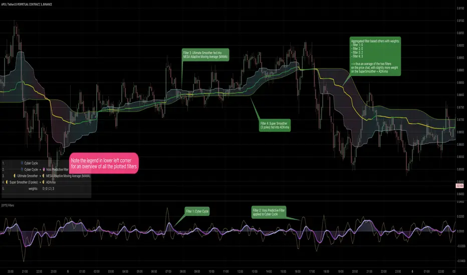
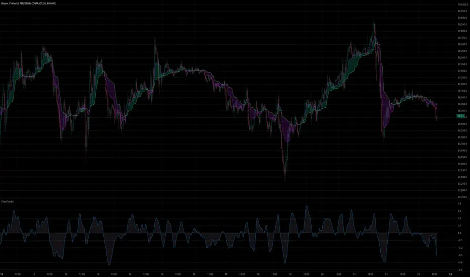
[GYTS] Filters ToolkitFilters Toolkit indicator
🌸 Part of GoemonYae Trading System (GYTS) 🌸
🌸 --------- 1. INTRODUCTION --------- 🌸
💮 Overview
The GYTS Filters Toolkit indicator is an advanced, interactive interface built atop the high‐performance, curated functions provided by the FiltersToolkit library . It allows traders to experiment with different combinations of filtering methods -— from smoothing low-pass filters to aggressive detrenders. With this toolkit, you can build custom indicators tailored to your specific trading strategy, whether you're looking for trend following, mean reversion, or cycle identification approaches.
🌸 --------- 2. FILTER METHODS AND TYPES --------- 🌸
💮 Filter categories
The available filters fall into four main categories, each marked with a distinct symbol:
🌗 Low Pass Filters (Smoothers)
These filters attenuate high-frequency components (noise) while allowing low-frequency components (trends) to pass through. Examples include:
Ultimate Smoother
Super Smoother (2-pole and 3-pole variants)
MESA Adaptive Moving Average (MAMA) and Following Adaptive Moving Average (FAMA)
BiQuad Low Pass Filter
ADXvma (Adaptive Directional Volatility Moving Average)
A2RMA (Adaptive Autonomous Recursive Moving Average)
Low pass filters are displayed on the price chart by default, as they follow the overall price movement. If they are combined with a high-pass or bandpass filter, they will be displayed in the subgraph.
🌓 High Pass Filters (Detrenders)
These filters do the opposite of low pass filters - they remove low-frequency components (trends) while allowing high-frequency components to pass through. Examples include:
Butterworth High Pass Filter
BiQuad High Pass Filter
High pass filters are displayed as oscillators in the subgraph below the price chart, as they fluctuate around a zero line.
🌑 Band Pass Filters (Cycle Isolators)
These filters combine aspects of both low and high pass filters, isolating specific frequency ranges while attenuating both higher and lower frequencies. Examples include:
Ehlers Bandpass Filter
Cyber Cycle
Relative Vigor Index (RVI)
BiQuad Bandpass Filter
Band pass filters are also displayed as oscillators in a separate panel.
🔮 Predictive Filter
Voss Predictive Filter: A special filter that attempts to predict future values of band-limited signals (only to be used as post-filter). Keep its prediction horizon short (1–3 bars) for reasonable accuracy.
Note that the the library contains elaborate documentation and source material of each filter.
🌸 --------- 3. INDICATOR FEATURES --------- 🌸
💮 Multi-filter configuration
One of the most powerful aspects of this indicator is the ability to configure multiple filters. compare them and observe their combined effects. There are four primary filters, each with its own parameter settings.
💮 Post-filtering
Process a filter’s output through an additional filter by enabling the post-filter option. This creates a filter chain where the output of one filter becomes the input to another. Some powerful combinations include:
Ultimate Smoother → MAMA: Creates an adaptive smoothing effect that responds well to market changes, good for trend-following strategies
Butterworth → Super Smoother → Butterworth: Produces a well-behaved oscillator with minimal phase distortion, John Ehlers also calls a "roofing filter". Great for identifying overbought/oversold conditions with minimal lag.
A bandpass filter → Voss Prediction filter: Attempts to predict future movements of cyclical components, handy to find peaks and troughs of the market cycle.
💮 Aggregate filters
Arguably the coolest feature: aggregating filters allow you to combine multiple filters with different weights. Important notes about aggregation:
You can only aggregate filters that appear on the same chart (price chart or oscillator panel).
The weights are automatically normalised, so only their relative values matter
Setting a weight to 0 (zero) excludes that filter from the aggregation
Filters don't need to be visibly displayed to be included in aggregation
💮 Rich visualisation & alerts
The indicator intelligently determines whether a filter is displayed on the price chart or in the subgraph (as an oscillator) based on its characteristics.
Dynamic colour palettes, adjustable line widths, transparency, and custom fill between any of enabled filters or between oscillators and the zero-line.
A clear legend showing which filters are active and how they're configured
Alerts for direction changes and crossovers of all filters
🌸 --------- 4. ACKNOWLEDGEMENTS --------- 🌸
This toolkit builds on the work of numerous pioneers in technical analysis and digital signal processing:
John Ehlers, whose groundbreaking research forms the foundation of many filters.
Robert Bristow-Johnson for the BiQuad filter formulations.
The TradingView community, especially @The_Peaceful_Lizard, @alexgrover, and others mentioned in the code of the library.
Everyone who has provided feedback, testing and support!
[GYTS] FiltersToolkit LibraryFiltersToolkit Library
🌸 Part of GoemonYae Trading System (GYTS) 🌸
🌸 --------- 1. INTRODUCTION --------- 🌸
💮 What Does This Library Contain?
This library is a curated collection of high-performance digital signal processing (DSP) filters and auxiliary functions designed specifically for financial time series analysis. It includes a shortlist of our favourite and best performing filters — each rigorously tested and selected for their responsiveness, minimal lag and robustness in diverse market conditions. These tools form an integral part of the GoemonYae Trading System (GYTS), chosen for their unique characteristics in handling market data.
The library contains two main categories:
1. Smoothing filters (low-pass filters and moving averages) for e.g. denoising, trend following
2. Detrending tools (high-pass and band-pass filters, known as "oscillators") for e.g. mean reversion
This collection is finely tuned for practical trading applications and is therefore not meant to be exhaustive. However, will continue to expand as we discover and validate new filtering techniques. I welcome collaboration and suggestions for novel approaches.
🌸 ——— 2. ADDED VALUE ——— 🌸
💮 Unified syntax and comprehensive documentation
The FiltersToolkit Library brings together a wide array of valuable filters under a unified, intuitive syntax. Each function is thoroughly documented, with clear explanations and academic sources that underline the mathematical rigour behind the methods. This level of documentation not only facilitates integration into trading strategies but also helps underlying the underlying concepts and rationale.
💮 Optimised performance and readability
The code prioritizes computational efficiency while maintaining readability. Key optimizations include:
- Minimizing redundant calculations in recursive filters
- Smart coefficient caching
- Efficient state management
- Vectorized operations where applicable
💮 Enhanced functionality and flexibility
Some filters in this library introduce extended functionality beyond the original publications. For instance, the MESA Adaptive Moving Average (MAMA) and Ehlers’ Combined Bandpass Filter incorporate multiple variations found in the literature, thereby providing traders with flexible tools that can be fine-tuned to different market conditions.
🌸 ——— 3. THE FILTERS ——— 🌸
💮 Hilbert Transform Function
This function implements the Hilbert Transform as utilised by John Ehlers. It converts a real-valued time series into its analytic signal, enabling the extraction of instantaneous phase and frequency information—an essential step in adaptive filtering.
Source: John Ehlers - "Rocket Science for Traders" (2001), "TASC 2001 V. 19:9", "Cybernetic Analysis for Stocks and Futures" (2004)
💮 Homodyne Discriminator
By leveraging the Hilbert Transform, this function computes the dominant cycle period through a Homodyne Discriminator. It extracts the in-phase and quadrature components of the signal, facilitating a robust estimation of the underlying cycle characteristics.
Source: John Ehlers - "Rocket Science for Traders" (2001), "TASC 2001 V. 19:9", "Cybernetic Analysis for Stocks and Futures" (2004)
💮 MESA Adaptive Moving Average (MAMA)
An advanced dual-stage adaptive moving average, this function outputs both the MAMA and its companion FAMA. It combines adaptive alpha computation with elements from Kaufman’s Adaptive Moving Average (KAMA) to provide a responsive and reliable trend indicator.
Source: John Ehlers - "Rocket Science for Traders" (2001), "TASC 2001 V. 19:9", "Cybernetic Analysis for Stocks and Futures" (2004)
💮 BiQuad Filters
A family of second-order recursive filters offering exceptional control over frequency response:
- High-pass filter for detrending
- Low-pass filter for smooth trend following
- Band-pass filter for cycle isolation
The quality factor (Q) parameter allows fine-tuning of the resonance characteristics, making these filters highly adaptable to different market conditions.
Source: Robert Bristow-Johnson's Audio EQ Cookbook, implemented by @The_Peaceful_Lizard
💮 Relative Vigor Index (RVI)
This filter evaluates the strength of a trend by comparing the closing price to the trading range. Operating similarly to a band-pass filter, the RVI provides insights into market momentum and potential reversals.
Source: John Ehlers – “Cybernetic Analysis for Stocks and Futures” (2004)
💮 Cyber Cycle
The Cyber Cycle filter emphasises market cycles by smoothing out noise and highlighting the dominant cyclical behaviour. It is particularly useful for detecting trend reversals and cyclical patterns in the price data.
Source: John Ehlers – “Cybernetic Analysis for Stocks and Futures” (2004)
💮 Butterworth High Pass Filter
Inspired by the classical Butterworth design, this filter achieves a maximally flat magnitude response in the passband while effectively removing low-frequency trends. Its design minimises phase distortion, which is vital for accurate signal interpretation.
Source: John Ehlers – “Cybernetic Analysis for Stocks and Futures” (2004)
💮 2-Pole SuperSmoother
Employing a two-pole design, the SuperSmoother filter reduces high-frequency noise with minimal lag. It is engineered to preserve trend integrity while offering a smooth output even in noisy market conditions.
Source: John Ehlers – “Cybernetic Analysis for Stocks and Futures” (2004)
💮 3-Pole SuperSmoother
An extension of the 2-pole design, the 3-pole SuperSmoother further attenuates high-frequency noise. Its additional pole delivers enhanced smoothing at the cost of slightly increased lag.
Source: John Ehlers – “Cybernetic Analysis for Stocks and Futures” (2004)
💮 Adaptive Directional Volatility Moving Average (ADXVma)
This adaptive moving average adjusts its smoothing factor based on directional volatility. By combining true range and directional movement measurements, it remains exceptionally flat during ranging markets and responsive during directional moves.
Source: Various implementations across platforms, unified and optimized
💮 Ehlers Combined Bandpass Filter with Automated Gain Control (AGC)
This sophisticated filter merges a highpass pre-processing stage with a bandpass filter. An integrated Automated Gain Control normalises the output to a consistent range, while offering both regular and truncated recursive formulations to manage lag.
Source: John F. Ehlers – “Truncated Indicators” (2020), “Cycle Analytics for Traders” (2013)
💮 Voss Predictive Filter
A forward-looking filter that predicts future values of a band-limited signal in real time. By utilising multiple time-delayed feedback terms, it provides anticipatory coupling and delivers a short-term predictive signal.
Source: John Ehlers - "A Peek Into The Future" (TASC 2019-08)
💮 Adaptive Autonomous Recursive Moving Average (A2RMA)
This filter dynamically adjusts its smoothing through an adaptive mechanism based on an efficiency ratio and a dynamic threshold. A double application of an adaptive moving average ensures both responsiveness and stability in volatile and ranging markets alike. Very flat response when properly tuned.
Source: @alexgrover (2019)
💮 Ultimate Smoother (2-Pole)
The Ultimate Smoother filter is engineered to achieve near-zero lag in its passband by subtracting a high-pass response from an all-pass response. This creates a filter that maintains signal fidelity at low frequencies while effectively filtering higher frequencies at the expense of slight overshooting.
Source: John Ehlers - TASC 2024-04 "The Ultimate Smoother"
Note: This library is actively maintained and enhanced. Suggestions for additional filters or improvements are welcome through the usual channels. The source code contains a list of tested filters that did not make it into the curated collection.
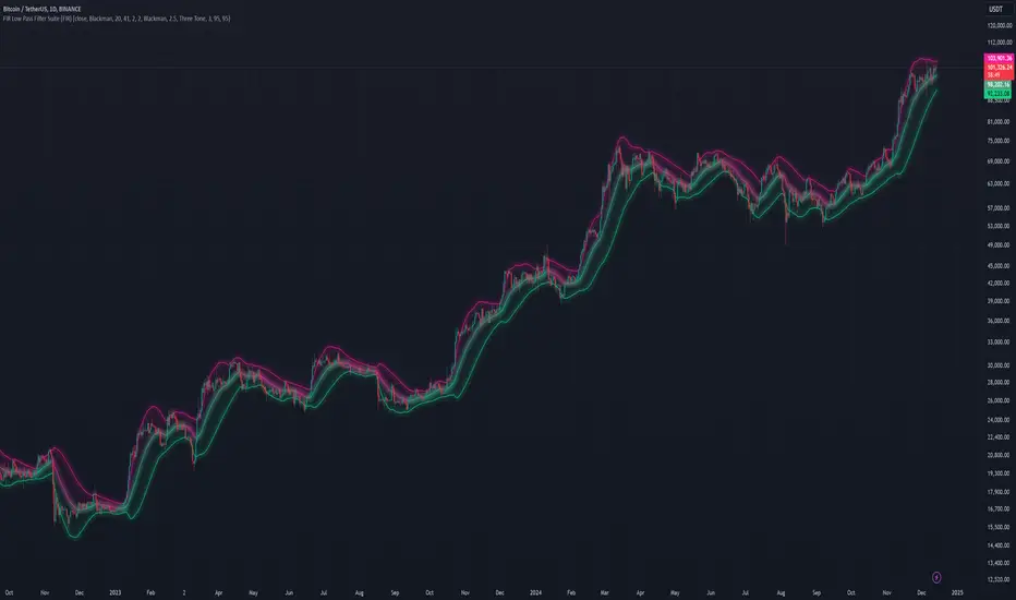
FIR Low Pass Filter Suite (FIR)The FIR Low Pass Filter Suite is an advanced signal processing indicator that applies finite impulse response (FIR) filtering techniques to price data. At its core, the indicator uses windowed-sinc filtering, which provides optimal frequency response characteristics for separating trend from noise in financial data.
The indicator offers multiple window functions including Kaiser, Kaiser-Bessel Derived (KBD), Hann, Hamming, Blackman, Triangular, and Lanczos. Each window type provides different trade-offs between main-lobe width and side-lobe attenuation, allowing users to fine-tune the frequency response characteristics of the filter. The Kaiser and KBD windows provide additional control through an alpha parameter that adjusts the shape of the window function.
A key feature is the ability to operate in either linear or logarithmic space. Logarithmic filtering can be particularly appropriate for financial data due to the multiplicative nature of price movements. The indicator includes an envelope system that can adaptively calculate bands around the filtered price using either arithmetic or geometric deviation, with separate controls for upper and lower bands to account for the asymmetric nature of market movements.
The implementation handles edge effects through proper initialization and offers both centered and forward-only filtering modes. Centered mode provides zero phase distortion but introduces lag, while forward-only mode operates causally with no lag but introduces some phase distortion. All calculations are performed using vectorized operations for efficiency, with carefully designed state management to handle the filter's warm-up period.
Visual feedback is provided through customizable color gradients that can reflect the current trend direction, with optional glow effects and background fills to enhance visibility. The indicator maintains high numerical precision throughout its calculations while providing smooth, artifact-free output suitable for both analysis and visualization.
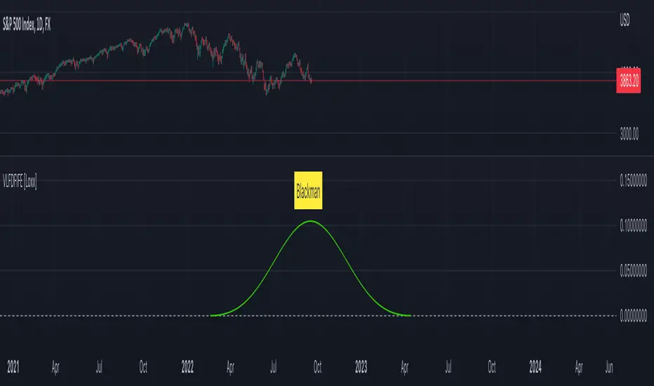
Variety, Low-Pass, FIR Filter Impulse Response Explorer [Loxx]Variety Low-Pass FIR Filter, Impulse Response Explorer is a simple impulse response explorer of 16 of the most popular FIR digital filtering windowing techniques. Y-values are the values of the coefficients produced by the selected algorithms; X-values are the index of sample. This indicator also allows you to turn on Sinc Windowing for all window types except for Rectangular, Triangular, and Linear. This is an educational indicator to demonstrate the differences between popular FIR filters in terms of their coefficient outputs. This is also used to compliment other indicators I've published or will publish that implement advanced FIR digital filters (see below to find applicable indicators).
Inputs:
Number of Coefficients to Calculate = Sample size; for example, this would be the period used in SMA or WMA
FIR Digital Filter Type = FIR windowing method you would like to explore
Multiplier (Sinc only) = applies a multiplier effect to the Sinc Windowing
Frequency Cutoff = this is necessary to smooth the output and get rid of noise. the lower the number, the smoother the output.
Turn on Sinc? = turn this on if you want to convert the windowing function from regular function to a Windowed-Sinc filter
Order = This is used for power of cosine filter only. This is the N-order, or depth, of the filter you wish to create.
What are FIR Filters?
In discrete-time signal processing, windowing is a preliminary signal shaping technique, usually applied to improve the appearance and usefulness of a subsequent Discrete Fourier Transform. Several window functions can be defined, based on a constant (rectangular window), B-splines, other polynomials, sinusoids, cosine-sums, adjustable, hybrid, and other types. The windowing operation consists of multipying the given sampled signal by the window function. For trading purposes, these FIR filters act as advanced weighted moving averages.
A finite impulse response (FIR) filter is a filter whose impulse response (or response to any finite length input) is of finite duration, because it settles to zero in finite time. This is in contrast to infinite impulse response (IIR) filters, which may have internal feedback and may continue to respond indefinitely (usually decaying).
The impulse response (that is, the output in response to a Kronecker delta input) of an Nth-order discrete-time FIR filter lasts exactly {\displaystyle N+1}N+1 samples (from first nonzero element through last nonzero element) before it then settles to zero.
FIR filters can be discrete-time or continuous-time, and digital or analog.
A FIR filter is (similar to, or) just a weighted moving average filter, where (unlike a typical equally weighted moving average filter) the weights of each delay tap are not constrained to be identical or even of the same sign. By changing various values in the array of weights (the impulse response, or time shifted and sampled version of the same), the frequency response of a FIR filter can be completely changed.
An FIR filter simply CONVOLVES the input time series (price data) with its IMPULSE RESPONSE. The impulse response is just a set of weights (or "coefficients") that multiply each data point. Then you just add up all the products and divide by the sum of the weights and that is it; e.g., for a 10-bar SMA you just add up 10 bars of price data (each multiplied by 1) and divide by 10. For a weighted-MA you add up the product of the price data with triangular-number weights and divide by the total weight.
What's a Low-Pass Filter?
A low-pass filter is the type of frequency domain filter that is used for smoothing sound, image, or data. This is different from a high-pass filter that is used for sharpening data, images, or sound.
Whats a Windowed-Sinc Filter?
Windowed-sinc filters are used to separate one band of frequencies from another. They are very stable, produce few surprises, and can be pushed to incredible performance levels. These exceptional frequency domain characteristics are obtained at the expense of poor performance in the time domain, including excessive ripple and overshoot in the step response. When carried out by standard convolution, windowed-sinc filters are easy to program, but slow to execute.
The sinc function sinc (x), also called the "sampling function," is a function that arises frequently in signal processing and the theory of Fourier transforms.
In mathematics, the historical unnormalized sinc function is defined for x ≠ 0 by
sinc x = sinx / x
In digital signal processing and information theory, the normalized sinc function is commonly defined for x ≠ 0 by
sinc x = sin(pi * x) / (pi * x)
For our purposes here, we are used a normalized Sinc function
Included Windowing Functions
N-Order Power-of-Cosine (this one is really N-different types of FIR filters)
Hamming
Hanning
Blackman
Blackman Harris
Blackman Nutall
Nutall
Bartlet Zero End Points
Bartlet-Hann
Hann
Sine
Lanczos
Flat Top
Rectangular
Linear
Triangular
If you wish to dive deeper to get a full explanation of these windowing functions, see here: en.wikipedia.org
Related indicators
STD-Filtered, Variety FIR Digital Filters w/ ATR Bands
STD/C-Filtered, N-Order Power-of-Cosine FIR Filter
STD/C-Filtered, Truncated Taylor Family FIR Filter
STD/Clutter-Filtered, Kaiser Window FIR Digital Filter
STD/Clutter Filtered, One-Sided, N-Sinc-Kernel, EFIR Filt
Ehlers Two-Pole Predictor [Loxx]Ehlers Two-Pole Predictor is a new indicator by John Ehlers . The translation of this indicator into PineScript™ is a collaborative effort between @cheatcountry and I.
The following is an excerpt from "PREDICTION" , by John Ehlers
Niels Bohr said “Prediction is very difficult, especially if it’s about the future.”. Actually, prediction is pretty easy in the context of technical analysis . All you have to do is to assume the market will behave in the immediate future just as it has behaved in the immediate past. In this article we will explore several different techniques that put the philosophy into practice.
LINEAR EXTRAPOLATION
Linear extrapolation takes the philosophical approach quite literally. Linear extrapolation simply takes the difference of the last two bars and adds that difference to the value of the last bar to form the prediction for the next bar. The prediction is extended further into the future by taking the last predicted value as real data and repeating the process of adding the most recent difference to it. The process can be repeated over and over to extend the prediction even further.
Linear extrapolation is an FIR filter, meaning it depends only on the data input rather than on a previously computed value. Since the output of an FIR filter depends only on delayed input data, the resulting lag is somewhat like the delay of water coming out the end of a hose after it supplied at the input. Linear extrapolation has a negative group delay at the longer cycle periods of the spectrum, which means water comes out the end of the hose before it is applied at the input. Of course the analogy breaks down, but it is fun to think of it that way. As shown in Figure 1, the actual group delay varies across the spectrum. For frequency components less than .167 (i.e. a period of 6 bars) the group delay is negative, meaning the filter is predictive. However, the filter has a positive group delay for cycle components whose periods are shorter than 6 bars.
Figure 1
Here’s the practical ramification of the group delay: Suppose we are projecting the prediction 5 bars into the future. This is fine as long as the market is continued to trend up in the same direction. But, when we get a reversal, the prediction continues upward for 5 bars after the reversal. That is, the prediction fails just when you need it the most. An interesting phenomenon is that, regardless of how far the extrapolation extends into the future, the prediction will always cross the signal at the same spot along the time axis. The result is that the prediction will have an overshoot. The amplitude of the overshoot is a function of how far the extrapolation has been carried into the future.
But the overshoot gives us an opportunity to make a useful prediction at the cyclic turning point of band limited signals (i.e. oscillators having a zero mean). If we reduce the overshoot by reducing the gain of the prediction, we then also move the crossing of the prediction and the original signal into the future. Since the group delay varies across the spectrum, the effect will be less effective for the shorter cycles in the data. Nonetheless, the technique is effective for both discretionary trading and automated trading in the majority of cases.
EXPLORING THE CODE
Before we predict, we need to create a band limited indicator from which to make the prediction. I have selected a “roofing filter” consisting of a High Pass Filter followed by a Low Pass Filter. The tunable parameter of the High Pass Filter is HPPeriod. Think of it as a “stone wall filter” where cycle period components longer than HPPeriod are completely rejected and cycle period components shorter than HPPeriod are passed without attenuation. If HPPeriod is set to be a large number (e.g. 250) the indicator will tend to look more like a trending indicator. If HPPeriod is set to be a smaller number (e.g. 20) the indicator will look more like a cycling indicator. The Low Pass Filter is a Hann Windowed FIR filter whose tunable parameter is LPPeriod. Think of it as a “stone wall filter” where cycle period components shorter than LPPeriod are completely rejected and cycle period components longer than LPPeriod are passed without attenuation. The purpose of the Low Pass filter is to smooth the signal. Thus, the combination of these two filters forms a “roofing filter”, named Filt, that passes spectrum components between LPPeriod and HPPeriod.
Since working into the future is not allowed in EasyLanguage variables, we need to convert the Filt variable to the data array XX. The data array is first filled with real data out to “Length”. I selected Length = 10 simply to have a convenient starting point for the prediction. The next block of code is the prediction into the future. It is easiest to understand if we consider the case where count = 0. Then, in English, the next value of the data array is equal to the current value of the data array plus the difference between the current value and the previous value. That makes the prediction one bar into the future. The process is repeated for each value of count until predictions up to 10 bars in the future are contained in the data array. Next, the selected prediction is converted from the data array to the variable “Prediction”. Filt is plotted in Red and Prediction is plotted in yellow.
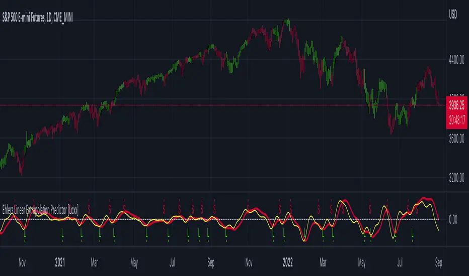
The Predict Extrapolation indicator is shown below for the Emini S&P Futures contract using the default input parameters. Filt is plotted in red and Predict is plotted in yellow. The crossings of the Predict and Filt lines provide reliable buy and sell timing signals. There is some overshoot for the shorter cycle periods, for example in February and March 2021, but the only effect is a late timing signal. Further reducing the gain and/or reducing the BarsFwd inputs would provide better timing signals during this period.
Figure 2. Predict Extrapolation Provides Reliable Timing Signals
I have experimented with other FIR filters for predictions, but found none that had a significant advantage over linear extrapolation.
MESA
MESA is an acronym for Maximum Entropy Spectral Analysis. Conceptually, it removes spectral components until the residual is left with maximum entropy. It does this by forming an all-pole filter whose order is determined by the selected number of coefficients. It maximally addresses the data within the selected window and ignores all other data. Its resolution is determined only by the number of filter coefficients selected. Since the resulting filter is an IIR filter, a prediction can be formed simply by convolving the filter coefficients with the data. MESA is one of the few, if not the only way to practically determine the coefficients of a higher order IIR filter. Discussion of MESA is beyond the scope of this article.
TWO POLE IIR FILTER
While the coefficients of a higher order IIR filter are difficult to compute without MESA, it is a relatively simple matter to compute the coefficients of a two pole IIR filter.
(Skip this paragraph if you don’t care about DSP) We can locate the conjugate pole positions parametrically in the Z plane in polar coordinates. Let the radius be QQ and the principal angle be 360 / P2Period. The first order component is 2*QQ*Cosine(360 / P2Period) and the second order component is just QQ2. Therefore, the transfer response becomes:
H(z) = 1 / (1 - 2*QQ*Cosine(360 / P2Period)*Z-1 + QQ2*Z-2)
By mixing notation we can easily convert the transfer response to code.
Output / Input = 1 / (1 - 2*QQ*Cosine(360 / P2Period)* + QQ2* )
Output - 2*QQ*Cosine(360 / P2Period)*Output + QQ2*Output = Input
Output = Input + 2*QQ*Cosine(360 / P2Period)*Output - QQ2*Output
The Two Pole Predictor starts by computing the same “roofing filter” design as described for the Linear Extrapolation Predictor. The HPPeriod and LPPeriod inputs adjust the roofing filter to obtain the desired appearance of an indicator. Since EasyLanguage variables cannot be extended into the future, the prediction process starts by loading the XX data array with indicator data up to the value of Length. I selected Length = 10 simply to have a convenient place from which to start the prediction. The coefficients are computed parametrically from the conjugate pole positions and are normalized to their sum so the IIR filter will have unity gain at zero frequency.
The prediction is formed by convolving the IIR filter coefficients with the historical data. It is easiest to see for the case where count = 0. This is the initial prediction. In this case the new value of the XX array is formed by successively summing the product of each filter coefficient with its respective historical data sample. This process is significantly different from linear extrapolation because second order curvature is introduced into the prediction rather than being strictly linear. Further, the prediction is adaptive to market conditions because the degree of curvature depends on recent historical data. The prediction in the data array is converted to a variable by selecting the BarsFwd value. The prediction is then plotted in yellow, and is compared to the indicator plotted in red.
The Predict 2 Pole indicator is shown above being applied to the Emini S&P Futures contract for most of 2021. The default parameters for the roofing filter and predictor were used. By comparison to the Linear Extrapolation prediction of Figure 2, the Predict 2 Pole indicator has a more consistent prediction. For example, there is little or no overshoot in February or March while still giving good predictions in April and May.
Input parameters can be varied to adjust the appearance of the prediction. You will find that the indicator is relatively insensitive to the BarsFwd input. The P2Period parameter primarily controls the gain of the prediction and the QQ parameter primarily controls the amount of prediction lead during trending sections of the indicator.
TAKEAWAYS
1. A more or less universal band limited “roofing filter” indicator was used to demonstrate the predictors. The HPPeriod input parameter is used to control whether the indicator looks more like a trend indicator or more like a cycle indicator. The LPPeriod input parameter is used to control the smoothness of the indicator.
2. A linear extrapolation predictor is formed by adding the difference of the two most recent data bars to the value of the last data bar. The result is considered to be a real data point and the process is repeated to extend the prediction into the future. This is an FIR filter having a one bar negative group delay at zero frequency, but the group delay is not constant across the spectrum. This variable group delay causes the linear extrapolation prediction to be inconsistent across a range of market conditions.
3. The degree of prediction by linear extrapolation can be controlled by varying the gain of the prediction to reduce the overshoot to be about the same amplitude as the peak swing of the indicator.
4. I was unable to experimentally derive a higher order FIR filter predictor that had advantages over the simple linear extrapolation predictor.
5. A Two Pole IIR predictor can be created by parametrically locating the conjugate pole positions.
6. The Two Pole predictor is a second order filter, which allows curvature into the prediction, thus mitigating overshoot. Further, the curvature is adaptive because the prediction depends on previously computed prediction values.
7. The Two Pole predictor is more consistent over a range of market conditions.
ADDITIONS
Loxx's Expanded source types:
Library for expanded source types:
Explanation for expanded source types:
Three different signal types: 1) Prediction/Filter crosses; 2) Prediction middle crosses; and, 3) Filter middle crosses.
Bar coloring to color trend.
Signals, both Long and Short.
Alerts, both Long and Short.

Ehlers Linear Extrapolation Predictor [Loxx]Ehlers Linear Extrapolation Predictor is a new indicator by John Ehlers. The translation of this indicator into PineScript™ is a collaborative effort between @cheatcountry and I.
The following is an excerpt from "PREDICTION" , by John Ehlers
Niels Bohr said “Prediction is very difficult, especially if it’s about the future.”. Actually, prediction is pretty easy in the context of technical analysis. All you have to do is to assume the market will behave in the immediate future just as it has behaved in the immediate past. In this article we will explore several different techniques that put the philosophy into practice.
LINEAR EXTRAPOLATION
Linear extrapolation takes the philosophical approach quite literally. Linear extrapolation simply takes the difference of the last two bars and adds that difference to the value of the last bar to form the prediction for the next bar. The prediction is extended further into the future by taking the last predicted value as real data and repeating the process of adding the most recent difference to it. The process can be repeated over and over to extend the prediction even further.
Linear extrapolation is an FIR filter, meaning it depends only on the data input rather than on a previously computed value. Since the output of an FIR filter depends only on delayed input data, the resulting lag is somewhat like the delay of water coming out the end of a hose after it supplied at the input. Linear extrapolation has a negative group delay at the longer cycle periods of the spectrum, which means water comes out the end of the hose before it is applied at the input. Of course the analogy breaks down, but it is fun to think of it that way. As shown in Figure 1, the actual group delay varies across the spectrum. For frequency components less than .167 (i.e. a period of 6 bars) the group delay is negative, meaning the filter is predictive. However, the filter has a positive group delay for cycle components whose periods are shorter than 6 bars.
Figure 1
Here’s the practical ramification of the group delay: Suppose we are projecting the prediction 5 bars into the future. This is fine as long as the market is continued to trend up in the same direction. But, when we get a reversal, the prediction continues upward for 5 bars after the reversal. That is, the prediction fails just when you need it the most. An interesting phenomenon is that, regardless of how far the extrapolation extends into the future, the prediction will always cross the signal at the same spot along the time axis. The result is that the prediction will have an overshoot. The amplitude of the overshoot is a function of how far the extrapolation has been carried into the future.
But the overshoot gives us an opportunity to make a useful prediction at the cyclic turning point of band limited signals (i.e. oscillators having a zero mean). If we reduce the overshoot by reducing the gain of the prediction, we then also move the crossing of the prediction and the original signal into the future. Since the group delay varies across the spectrum, the effect will be less effective for the shorter cycles in the data. Nonetheless, the technique is effective for both discretionary trading and automated trading in the majority of cases.
EXPLORING THE CODE
Before we predict, we need to create a band limited indicator from which to make the prediction. I have selected a “roofing filter” consisting of a High Pass Filter followed by a Low Pass Filter. The tunable parameter of the High Pass Filter is HPPeriod. Think of it as a “stone wall filter” where cycle period components longer than HPPeriod are completely rejected and cycle period components shorter than HPPeriod are passed without attenuation. If HPPeriod is set to be a large number (e.g. 250) the indicator will tend to look more like a trending indicator. If HPPeriod is set to be a smaller number (e.g. 20) the indicator will look more like a cycling indicator. The Low Pass Filter is a Hann Windowed FIR filter whose tunable parameter is LPPeriod. Think of it as a “stone wall filter” where cycle period components shorter than LPPeriod are completely rejected and cycle period components longer than LPPeriod are passed without attenuation. The purpose of the Low Pass filter is to smooth the signal. Thus, the combination of these two filters forms a “roofing filter”, named Filt, that passes spectrum components between LPPeriod and HPPeriod.
Since working into the future is not allowed in EasyLanguage variables, we need to convert the Filt variable to the data array XX . The data array is first filled with real data out to “Length”. I selected Length = 10 simply to have a convenient starting point for the prediction. The next block of code is the prediction into the future. It is easiest to understand if we consider the case where count = 0. Then, in English, the next value of the data array is equal to the current value of the data array plus the difference between the current value and the previous value. That makes the prediction one bar into the future. The process is repeated for each value of count until predictions up to 10 bars in the future are contained in the data array. Next, the selected prediction is converted from the data array to the variable “Prediction”. Filt is plotted in Red and Prediction is plotted in yellow.
The Predict Extrapolation indicator is shown above for the Emini S&P Futures contract using the default input parameters. Filt is plotted in red and Predict is plotted in yellow. The crossings of the Predict and Filt lines provide reliable buy and sell timing signals. There is some overshoot for the shorter cycle periods, for example in February and March 2021, but the only effect is a late timing signal. Further reducing the gain and/or reducing the BarsFwd inputs would provide better timing signals during this period.
ADDITIONS
Loxx's Expanded source types:
Library for expanded source types:
Explanation for expanded source types:
Three different signal types: 1) Prediction/Filter crosses; 2) Prediction middle crosses; and, 3) Filter middle crosses.
Bar coloring to color trend.
Signals, both Long and Short.
Alerts, both Long and Short.
[DSPrated] Modified EMD for swing tradeModified Ehlers Empirical Mode Decomposition indicator for swing trade based on Butterworth 2nd order IIR filter
Description
This script is inspired by John Ehlers' TECHNICAL PAPERS - Truncating Indicators and Empirical Mode Decomposition. But instead of detecting trend it applies to finding swing regions.
Also here is suggested canonical DSP approach for designing coefficients for Butterworth 2nd order IIR filters - bandpass and lowpass.
Besides, truncated IIR filter with configurable length parameter is used. It worth mentioning, that although truncated filter is more robust than original IIR, it losses specified properties (bandpass) the more, the less is length parameter.
Butterworth Bandpass Infinite Impulse Response (IIR) Filter
This is the 2nd order Butterworth Bandpass Infinite Impulse Response (IIR) Filter based on the transform from the 1st order lowpass
Based on the example 8.8 on p476 from book Digital Signal Processing: A Practical Approach 2nd Edition by Emmanuel C. Ifeachor (Author), Barrie W. Jervis (Author)
It differs from Ehlers BandPass Filter only in the way you initialize input parameters. Here you can define cutoff periods of region of interest. For example on a timeframe, where one bar equals 1 hour you can define periods 18 and 22, which mean you'll see the swing intensity of price movement components within specified range.
Parameters
Source
Period 1 - cutoff period of bandpass begining
Period 2 - cutoff period of the end of bandpass
length - IIR truncation length
Concept of usage
Within specified bandpass this indicator eliminates the Trend line according to Ehlers EMD. The bandpass periods is recommended to choose accordingly to personal comfortable trading style and timeframe.
The trendline painted with 3 colors depending of the next modes:
up tend - green
cycling - black
downtrend - red
So the buy signal is generated when trend line in cycling mode and filtered component reaches it local minimum.
And the sell signal is generated when trend line in cycling mode and filtered component reaches it local maximum.
Secure long and short zones marked with color.
---
// TO DO
// - compare truncated and full version using signal generators
// - apply zero lag filter modification fordetectig ternd and swing peroids
// - implement strategy scripts
// - implement somewhat "true" EMD with sevral IMFs(intrinsic mode function)
// - better description?
// - parameter optimization
---
Please, feel free to report any issues and improvement suggestions.

Roofing Filter [DW]This is an experimental study built on the concept of using roofing filters on price data proposed by John Ehlers.
Roofing filters are a type of bandpass filter conventionally used in HF radio receivers in the first IF stage to limit the frequency spectrum passed on to later stages in the receiver.
The goal in applying roofing filters to a price signal is to simultaneously attenuate high frequency noise and low frequency distortion to pass an oscillating signal with a nearly zero mean for analysis and/or further calculation.
In this study, there are three filter types to choose from:
-> Ehlers Roofing Filter, which passes data through a 2 pole high pass filter, then through a Super Smoother filter.
-> Gaussian Roofing Filter, which passes data through a 2 pole Gaussian high pass filter, then through a 2 pole Gaussian low pass filter.
-> Butterworth Roofing Filter, which passes data through a 2 pole Butterworth high pass filter, then through a 2 pole Butterworth low pass filter.
Each filter type has different amplitude and delay characteristics, so play around with each type and see which response suits your needs best.
There is an option to normalize the scale of the output as well. The normalization process in this script is computed by comparing positive and negative outputs to the filter's moving RMS value.
The resulting oscillator can be fed through numerous conventional indicators including Stochastic Oscillator, RSI, CCI, etc. to generate smoother, less distorted indicators for a clearer view of turning points.
Alternatively, it can also act as an indicator itself, as implied by the corresponding color scheme included in the script.
Although roofing filters are not conventionally used in the analysis of market data, applying such spectral analysis techniques may prove to be quite useful for the design of more efficient indicators and more reliable predictions.

Low Pass Channel [DW]This is an experimental study designed to attenuate higher frequency oscillations in price and volatility with minimal lag.
In this study, a single pole low pass filter is used. The low pass filter's cutoff period is determined either by a fixed user input, or by using an Instantaneous Frequency Measurement (IFM) algorithm.
Most radar warning, electronic countermeasures, and electronic intelligence systems employ IFM to identify threats, map the electronic battlefield, and implement deceptive countermeasures.
The IFM technique used for this study was devised by John Ehlers. It calculates In Phase and Quadrature (IQ) components using the Hilbert Transform and uses them to determine the dominant price cycle.
To generate the channel, the same filter approach is applied to true range then added to and subtracted from the price filter.
Custom bar colors are included for simple wave and trend indication.

Recursive Median FilterRecursive Median Filter indicator script.
This indicator was originally developed by John F. Ehlers (Stocks & Commodities V. 36:03 (8–11): Recursive Median Filters).
Recursive Median OscillatorRecursive Median Oscillator indicator script.
This indicator was originally developed by John F. Ehlers (Stocks & Commodities V. 36:03 (8–11): Recursive Median Filters).

NG [All Moving Averages]Collection of some of the best moving averages.
I've tried to collect them all but TV became so slow, that it was completely unusable.
So i left only those that performs best on various backtest systems.
