OSOK - One Shot One Kill( Macros w/ Body Swings, SD Prj)What you get:
Time windows: contiguous 50→10 (HH:50–(HH+1):10) and 20→40 (HH:20–HH:40), or both.
Kill Zones & Day filter: Asian, London, NY, London Close; weekdays toggles.
Static projection TF: compute swings on 5-minute (or custom) and display on any chart TF.
Fibonacci/SD ladder: internal retracements & multi-SD extensions with optional price labels.
Stats table: per-hour counts, average/ min/ max range, plus hit-rates for +1/+2/+3/+4 and −1/−2.
Sequence logic (optional): track conditional paths (e.g., 0→+2, +1→−2, etc.) to separate continuation vs. reversal behavior.
CSV export: push current table (filtered/sorted) to a chart label for copy-out.
Fraktal

Universal Sentiment Score — V3 Bottom DetectorThe Universal Sentiment Score (USS) condenses a wide range of market conditions into one easy-to-read oscillator. Instead of relying on a single signal, USS blends multiple forms of trend strength, momentum behavior, volatility shifts, and reversal conditions to generate a unified sentiment metric.

Fractal Levels Monitor w/ Trade Lines (ChadAnt) v2Small update. Prevents the break candle from getting another signal after the first buy/sell signal detected.
1. Fractal Level Detection
The indicator identifies Fractals, which are simply a series of bars where the center bar has the highest high (Bearish Fractal) or the lowest low (Bullish Fractal) compared to a set number of bars on either side (determined by the "Fractal Period" input, usually 2 to 5 bars).
Bullish Fractal Level (Support): The indicator plots a horizontal line at the lowest low of the most recently formed Bullish Fractal.
Bearish Fractal Level (Resistance): It plots a horizontal line at the highest high of the most recently formed Bearish Fractal.
2. The "Cross Candle" Event
The core idea isn't to trade the fractal itself, but the reaction after the fractal level is broken.
When the price breaks and closes through the established Bullish Level (support) or Bearish Level (resistance), that bar is marked as the Cross Candle.
This Cross Candle's High and Low are saved. This is the "setup" for the trade.
3. The Trade Signal (Entry Trigger)
A trade is only taken when the price breaks the extreme (High or Low) of the Cross Candle.
Buy Signal: The trade is entered long if the price breaks above the High of the Cross Candle.
Sell Signal: The trade is entered short if the price breaks below the Low of the Cross Candle.

Fractal Levels Monitor w/ Trade Lines (ChadAnt)1. Fractal Level Detection
The indicator identifies Fractals, which are simply a series of bars where the center bar has the highest high (Bearish Fractal) or the lowest low (Bullish Fractal) compared to a set number of bars on either side (determined by the "Fractal Period" input, usually 2 to 5 bars).
Bullish Fractal Level (Support): The indicator plots a horizontal line at the lowest low of the most recently formed Bullish Fractal.
Bearish Fractal Level (Resistance): It plots a horizontal line at the highest high of the most recently formed Bearish Fractal.
2. The "Cross Candle" Event
The core idea isn't to trade the fractal itself, but the reaction after the fractal level is broken.
When the price breaks and closes through the established Bullish Level (support) or Bearish Level (resistance), that bar is marked as the Cross Candle.
This Cross Candle's High and Low are saved. This is the "setup" for the trade.
3. The Trade Signal (Entry Trigger)
A trade is only taken when the price breaks the extreme (High or Low) of the Cross Candle.
Buy Signal: The trade is entered long if the price breaks above the High of the Cross Candle.
Sell Signal: The trade is entered short if the price breaks below the Low of the Cross Candle.

Multi-Timeframe Pivot ZonesThis indicator plots dynamic support and resistance levels from higher timeframes onto your current chart. It calculates the high, low, midpoint, and quartile (25%, 75%) levels from up to four different higher timeframes, projecting them forward as potential reaction zones.
🔍 **KEY FEATURES:**
• **Multi-Timeframe Analysis:** View key levels from 4 different timeframes simultaneously
• **Smart Visibility:** Levels only appear on timeframes equal to or lower than their source
• **Customizable Styles:** Choose colors, line widths, and styles (solid, dashed, dotted) for each timeframe
• **Projected Zones:** Levels extend into the future to show potential support/resistance areas
⚙ **HOW TO USE:**
1. Enable/disable timeframes in the settings
2. Set each timeframe to match your trading strategy (e.g., 1H, 4H, D, W)
3. Watch for price reactions at these levels for entry/exit signals
4. Use the quartile levels (25%, 75%) as secondary support/resistance areas
The indicator helps traders identify confluence areas where multiple timeframes align, increasing the significance of potential reversal or breakout points.

Weekly expansion (CRT) This indicator is designed to be used primarily on the daily chart,to aid in spotting weekly expansions, its a blend of CRT Theory and some ICT concepts.

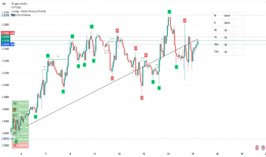
BACK TO BASIC, MTF, AOI, BOS Hiya ALL my Friends !!
I am going back to basic, MTF, AOI, BOS, mostly from freely available indicators, just adding the 8 TFs for reference. Hope this will simplify my analysis.
Cheers always !!
DYOR / NFA
Known Reversals (CreativeAdvance)1 min left to edit script
13 minutes ago
Known Reversals (CreativeAdvance)
Manage access
Add to favorites
Use on chart
0
0
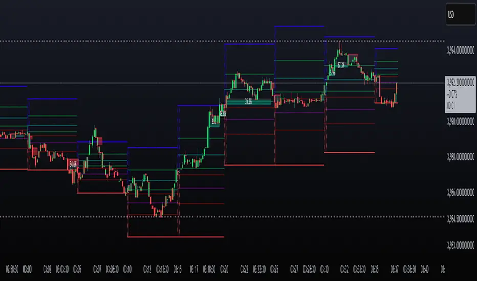
Known Reversals
Non-repainting 1-bar reversal detector
What it does:
Pinpoints the earliest confirmed reversals by detecting a subtle divergence within prevailing momentum. Delivers signals with zero lag and no repaint.
Core logic:
- Monitors directional momentum via highs in uptrends and lows in downtrends
- Activates only when the **close breaks alignment** with that momentum in a single candle
- Proprietary volatility-adjusted oscillator ensures signals fire exclusively in high-probability reversal contexts
Key advantage:
Reveals lower-timeframe reversals the moment they confirm on the current chart — true X-ray vision for precision entries.
Pro tip:
Use with distinct candlestick outline colors to instantly distinguish bullish vs. bearish signals, especially on inside bar reversals (painted uniformly for clarity).
No inputs. No curve-fitting. Just pure, actionable reversal confirmation.

VWAP D/W/M + MA100 & EMA100 albanThis TradingView indicator displays three independent VWAPs (Volume Weighted Average Prices) along with MA100 (Simple Moving Average) and EMA100 (Exponential Moving Average) on the chart.
Key Features:
VWAP #1, VWAP #2, VWAP #3: Each VWAP can be configured independently with:
Source (hlc3, close, etc.)
Anchor period (Session, Week, Month, Quarter, Year, Decade, Century, Earnings, Dividends, Splits)
Offset
Option to hide on daily or higher timeframes
MA100: 100-period Simple Moving Average
EMA100: 100-period Exponential Moving Average
Purpose:
This script is ideal for traders who want to track multiple VWAP levels simultaneously while also monitoring the 100-period moving averages for trend analysis. It provides a clean setup without bands or fills, focusing solely on price averages.
Use Cases:
Identify intraday or multi-timeframe VWAP levels
Combine VWAP levels with MA100/EMA100 for support/resistance analysis
Analyze trend direction and momentum using moving averages

Highlight Selected PeriodEdit and put what month or week you want and it will highlight all january's or all second weeks of the month to try and see if there are any patterns.

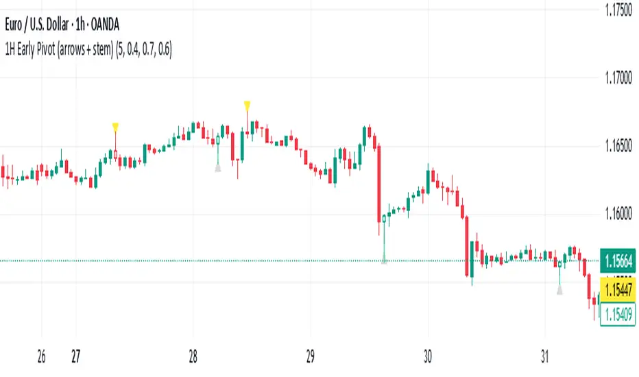
1H Early Pivot (arrows + stem) by Pastor CarrThis indicator helps to find early pivot points on the IH chart.
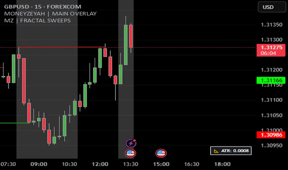
MZ | FRACTAL SWEEPSReady to LEVEL UP your trading game? Experience the power of real-time Fractal Sweeps and never let smart money trap you again! 🏦📈
Catch Explosive Moves: Instantly see when price sweeps key highs/lows and exposes where the real liquidity is hiding. No more chasing fakeouts or getting caught by surprise! 🎯
Turn Confusion into Clarity: Built for ALL traders — from scalpers to swing traders! Get crystal-clear signals on any market or timeframe. 🔍
Plug-and-Play: Easy to set up, works on stocks, crypto, forex… you name it! Universal edge for any chart. 🌍
Smart Visuals & Alerts: Vibrant sweep markers and powerful instant alerts keep you ahead, even if you step away. 🏃♂️💡
Backed by PRO Logic: Inspired by institutional trading — but accessible, visual, and actionable for everyone. 💪
If you want to stop blindly trading, and start outmanoeuvring the herd, this is for you. Jump in, stand out, and let your results do the talking! 🦁
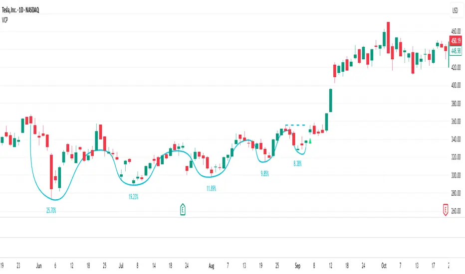
VCP Detector it detects VCP before breakout,,,
⚡ How to Use
🕒 Timeframe:
15-min → Intraday contraction
Daily → Swing contraction
🟢 Green circles = VCP zones
→ price tightening, volume drying, volatility compressing.

Volatility Contraction PatternThe Volatility Contraction Pattern (VCP), popularized by Mark Minervini, is a price-action formation that reflects supply drying up and institutional accumulation before a breakout. A proper VCP demonstrates a prior uptrend, constructive base development, sequential declines in downside volatility, and evidence of institutional accumulation.
This indicator identifies and tracks VCP behavior by mapping successive contraction legs (up to five), verifying that each pullback forms a higher low with diminishing depth, and highlighting when the final contraction tightens sufficiently relative to earlier legs. A dynamic pivot line highlights the key breakout level, and a confirmation trigger signals when price breaks above that pivot.
A classic VCP typically includes:
A strong prior uptrend into the base
2–5 tightening pullbacks (contractions) with higher lows
Decreasing volatility and often reduced volume
A clear pivot level (last swing high)
Breakout through the pivot as demand overwhelms supply
The psychology: early sellers are absorbed, weak holders exit, and stronger hands take control — setting up for a powerful upside move.
How This Indicator Identifies VCPs
This script automatically tracks price swings to detect VCP-style contraction sequences. It:
Anchors to an initial swing high and low
Identifies each subsequent contraction when price pulls back and then moves back up
Ensures each contraction is higher-low + shallower than the prior
Verifies a minimum contraction bar count to avoid noise
Tracks up to five contractions (C1 → C5)
Confirms a valid VCP when the final contraction tightens within a user-defined threshold
Marks the pivot (last contraction high)
Triggers a breakout signal when price exceeds that pivot
Indicator Settings & Features
Contraction Display
Plots each contraction leg and base structure
Supports curved or straight visual style
Optionally labels each contraction with its depth (% decline)
This helps quickly evaluate whether volatility is truly contracting.
Contraction Depth Controls
Maximum Depth — filters out patterns with overly deep first-leg pullbacks
Final Contraction Depth — requires the last pullback to be especially tight, as Minervini describes
This ensures the base tightens toward the right side — a key VCP principle.
Breakout Logic
Breakout confirms when price exceeds the pivot high
Triangle marker plots at breakout candle
Reset & Threshold Logic
A small threshold buffer prevents false pattern resets when price slightly exceeds highs
Auto-reset after excessive depth or extended time to avoid stale patterns
Alerts
VCP Forming when a qualifying contraction sequence completes
VCP Breakout when price clears the pivot

Monday to Friday MarkersDay of Week marker. True day open. Monday through friday times weekends not included

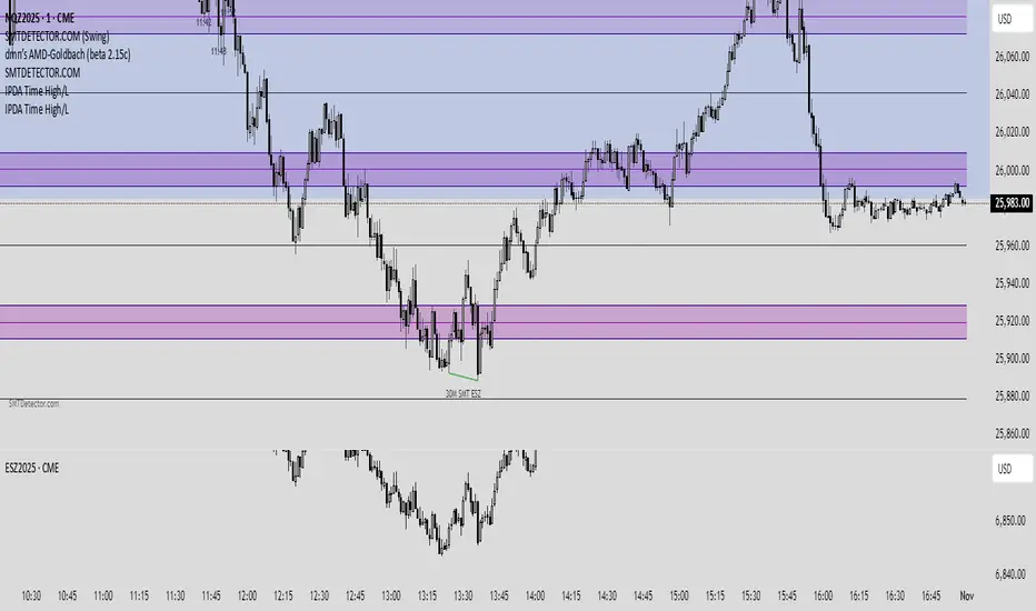
IPDA Time High/L🧭 IPDA Time Pivot High/Low (3•6•9)
Precision timing meets liquidity delivery.
🔹 Concept
This tool is built on the idea that price is delivered by time, not structure — a core belief in Zeussy/Smart Money–style analysis.
Certain time signatures, known as IPDA times (where the digits of hour and minute reduce to 3, 6, or 9), often align with reversals, traps, or accelerations in market delivery.
These times represent rhythmic energy cycles in algorithmic delivery, marking when liquidity is often redistributed.
🔹 What the Indicator Does
Scans your selected time window (default: 9:00–11:00, New York).
Identifies candles forming micro pivots — a candle that’s higher or lower than both its immediate neighbors.
Filters only those pivots that occur at IPDA times (digital roots of 3, 6, or 9).
Prints a clean, minimal time label (HH:MM) above or below each qualifying candle.
Labels dynamically adjust to your chart’s timezone and vertical spacing for clarity.
🔹 Why It’s Useful
These moments often align with:
Engineered traps during liquidity hunts.
Session transitions (e.g., London → NY Open).
Delivery shifts where price changes direction into the Draw on Liquidity (DOL).
By highlighting only precise, time-based pivots, this indicator helps traders:
Anticipate timing-based reversals,
Align narrative with smart-money delivery cycles,
And build refined entries within the NY AM session.
🔹 How to Use
Apply the indicator to your chart.
Set the timezone (default: America/New_York).
Focus on your session window (e.g., 09:00–11:00).
Observe when price reaches your POI or liquidity pool during an IPDA time — those candles are often where manipulation or delivery begins.
Combine with your own narrative tools (SMT, CISD, DOL, POI) for confirmation.
🔹 Features
Automatic timezone alignment
Adjustable session hours
Transparent, minimalistic time labels
Custom label size & offset for clean chart aesthetics
Works on all intraday timeframes
🔹 Philosophy
“Price is delivered by time, not structure.”
— Zeussy
This indicator was designed for traders who study timing as a function of delivery,
not just structure — allowing you to see when the algorithm intends to act.
NWOG/NDOG - HOKO (Public Version)This indicator shows you the intervals between the start of the week and the new day, and it is useful for everyone and everyone can use it.

Chart Info Display (HOKO) 2It displays 3 things on the screen in order: symbol, date, time frame. You can use it to capture educational videos to make your chart more beautiful, more private, and more practical.

Hoko Quarterly Theory is it this Quarterly Theory but for faraz................................................................................................................................................................................................................
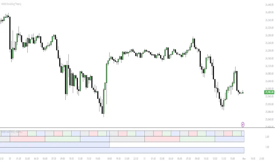
HOKO Doubling Theorythis script is like Quarterly theory but with bigger box .............................................................................................................................
