FLUX — Göstergeler ve Stratejiler

[GYTS-CE] Flux Composer 🧬 Flux Composer (Community Edition) 🌸 Confluence indicator in GoemonYae Trading System (GYTS) 🌸 The Flux Composer is a powerful tool in the GYTS suite that is designed to aggregate signals from multiple Signal Providers, apply customisable decaying functions, and offer customisable and advanced confluence mechanisms. This allows making informed decisions by considering the strength and agreement ("when all stars align") of various input signals. 🌸 --------- TABLE OF CONTENTS --------- 🌸 1️⃣ Main Highlights 2️⃣ Flux Composer’s Features Multi Signal Provider support Advanced decaying functions Customisable Flux confluence mechanisms Actionable trading experience User-friendly experience 3️⃣ User Guide Selecting Signal Providers Connecting Signal Providers to the Flux Composer Understanding the Flux Tuning the decaying functions Choosing Flux confluence mechanism Choosing sensitivity Interpreting the Flux for trading signals 4️⃣ Limitations 🌸 ------ 1️⃣ --- MAIN HIGHLIGHTS --- 1️⃣ ------ 🌸 - Signal aggregation : Combines signals from multiple different 📡 Signal Providers, each of which can be tuned and adjusted independently. - Decaying function : Utilises advanced decaying functions to model the diminishing effect of signals over time, ensuring that recent signals have more weight. In addition to the decaying effect, the "quality" of the original signals (e.g. a "strong" GDM from WaveTrend 4D with GDM ) are accounted for as well. - Flux confluence mechanism : The aggregation of all decaying functions form the "Flux", which is the core signal measurement of the Flux Composer. Multiple mechanisms are available for creating the Flux and effectively using it for actionable trading signals. - Visualisation : Provides detailed visualisation options to help users understand and tune the contributions of individual Signal Providers and their decaying functions. - Backtesting : The 🧬 Flux Composer is a core component of the TradingView suite of the 🌸 GoemonYae Trading System (GYTS) 🌸. It connects multiple 📡 Signal Providers, such as the WaveTrend 4D, and processes their signals to produce a unified "Flux". This Flux can then be used by the GYTS "🎼 Order Orchestrator" for backtesting and trade automation. 🌸 ------ 2️⃣ --- FLUX COMPOSER'S FEATURES --- 2️⃣ ------ 🌸 Let's delve into more details... 💮 1. Multi Signal Provider support Using the name of the GYTS "🎼 Order Orchestrator" as an analogy: Imagine a symphony where each instrument plays its own unique part, contributing to the overall harmony. The Flux Composer operates similarly, integrating multiple Signal Providers to create a comprehensive and robust trading signal -- the "Flux". Currently, it supports up to two streams from the WaveTrend 4D’s Gradient Divergence Measure (GDM) and another two streams from the WaveTrend 4D's Quantile Median Cross (QMC) . Note that the GDM includes 2 different continuous signals and the QMC 3 different continuous signals (from different frequencies). This means that the Community Edition can handle 2*2 + 2*3 = 10 different continuous signals. As GYTS evolves, more Signal Providers will be added; at the moment of releasing the Flux Composer, only WaveTrend 4D with GDM and with QMC are publicly available. 💮 2. Advanced decaying functions A trading signal can be relevant today, less relevant tomorrow, and irrelevant in a week's time. In other words, its relevance diminishes, or decays , over time. The Flux Composer utilises decaying functions that ensure that recent signals carry more weight, while older signals fade away. This is crucial for accurate signal processing. The intensity and decay settings allow for precise control, allowing emphasising certain signals based on their strength and relevance over time. On top of that, unlike binary signals ("buy now"), the Flux Composer utilises the actual values from the Signal Providers, differentiating between the exact quality of signals, and thus offering a detailed representation of the trading landscape. We will illustrate this in a further section. 💮 3. Customisable Flux confluence mechanisms Another core component of the Flux Composer is the ability of intelligently combining the decaying functions. It offers two sophisticated confluence mechanisms: Amplitude Compression and Trigonometric. Each mechanism has its unique way of processing the Flux, tailored to different trading needs. The Amplitude Compression method scales the Flux based on recent values, much like the Stochastic Oscillator, while the Trigonometric method uses smooth functions to reduce outliers’ impact We'll discuss this in more detail in the User Guide section. 💮 4. Actionable trading experience While the mathematical abilities might seem overwhelming, the goal of the Flux Composer is to transform complex signal data into actionable trading signals. When the Flux reaches certain thresholds, it generates clear bullish or bearish signals, making it easy for traders to interpret. The inclusion of upper and lower thresholds (UT and LT) helps in identifying strong signals visually and should be a familiar behaviour similar to how many other indicators operate. Furthermore, the Flux Composer can plot trading signals directly on the oscillator, showing triangle shapes for buy or sell signals. This visual aid is complemented by the possibility to setup TradingView alerts. 💮 5. User-friendly experience GYTS is all about sophisticated, robust methods but also "elegance". One of the interpretations of the latter, is that the users' experience is very important. Despite the Flux Composer's mathematical underpinnings, it offers intuitive settings that with omprehensive tooltips to help with a smooth setup process. For those looking to fine-tune their signals, the Flux Composer allows the visualisation of individual decaying functions. This feature helps users understand the impact of each setting and make informed adjustments. 🌸 ------ 3️⃣ --- USER GUIDE --- 3️⃣ ------ 🌸 💮 1. Selecting Signal Providers The Flux Composer’s foundation lies in its Signal Providers. When starting with the Flux Composer, using a single Signal Provider can already provide significant value due to the nature of decaying functions. For instance, the WaveTrend 4D signal provider includes up to two GDM and three QMC signals in a single direction (long/short). Moreover, the various confluence mechanisms that enhance the resulting Flux result in improved discrimination between weak and strong signals. This approach is akin to ensemble learning in machine learning, where multiple models are combined to improve predictive performance. While using a single Signal Provider is beneficial, the true power of the Flux Composer is realised with multiple Signal Providers. Here are two general approaches to selecting Signal Providers: Diverse Behaviours Use Signal Providers with different behaviours, such as WaveTrend 4D on various assets/timeframes or entirely different Signal Providers. This approach leverages diversification to achieve robustness, rooted in the principle that varied sources enhance the overall signal quality. To explain this with an analogy, this strategy aligns with the theory of diversification in portfolio management, where combining uncorrelated assets reduces overall risk. Similarly, combining uncorrelated signals can mitigate the risk of signal failure. A practical example can be integrating a mean-reversion signal with a trend-following signal -- these can balance each other out, providing more stable outputs over different market conditions. Enhancing a Single Provider If you consider a particular Signal Provider highly effective, you could improve its robustness by using multiple instances with slight variations. These variations could include different sources (e.g., close, HL2, HLC3), data providers (same asset across different brokers/exchanges), or parameter adjustments. This method mirrors Monte Carlo simulations, often used in risk management and derivative pricing, which involve running many simulations with varied inputs to estimate the probability of different outcomes. By applying similar principles, the strategy becomes less susceptible to overfitting, ensuring the signals are not overly dependent on specific data conditions. 💮 2. Connecting Signal Providers to the Flux Composer Moving on to practicalities: how do you connect Signal Providers with the Flux Composer? You may have noticed that when you open the drawdown of a data source in a TradingView indicator (with "open", "high", "low", etc.), you also see names from other indicators on your chart. We call these "streams", and the Signal Providers are designed such that they output this stream in a way that the Flux Composer can interpret it. Thus, to connect a Signal Provider with the Flux Composer, you should first have that Signal Provider on your chart. Obviously you should set it up an a way that it seems to provide good signals. After that, in the Data Stream dropdown in the Flux Composer, you can select the stream that is outputted by your Signal Provider. This will always be with a prefix of "🔗 STREAM" (after the Signal Provider's indicator name). See the chart below. There is one important nuance: when you have multiple (similar) Signal Providers on your chart, it may be hard to select the correct data stream in the Flux Composer as the names of the streams keep repeating when you use identical indicators. So be sure to be attentive as you might end up using the same signals multiple times. Also, the Signal Providers have an "Indicator name" parameter (and another parameter to repeat this name) that is handy to use when you have multiple Signal Providers on your screen. It is handy to give names that describe the unique settings of that Signal Provider so you can better differentiate what you are looking at on your screen. 💮 3. Understanding the Flux Let's understand how the Signal Provider's signals are processed. In the chart below, you see we have one Signal Provider (WaveTrend 4D) connected to the Flux Composer and that it gives a bearish QMC signal. The Flux Composer converts this into a decaying function. You can show these functions per Signal Provider when the option "Show decaying function of Signal Provider" is enabled (as it is in the chart). In our opinion, of crucial importance is the ability to process the quality of signals, rather than just any signal. In mathematical terms, we are interested in continuous signals as these provide a spectrum of values. These signals can reflect varying degrees of market sentiment or trend strength, offering richer information than binary signals, which offer only two states (e.g., buy/sell). Especially in the context of the Flux Composer, where you aggregate multiple signals, it makes a big difference whether you combine 10 weak signals or 10 strong signals. To illustrate this principle, look at the chart below where there are 4 signals of different strengths. As you can see, each of the signals affects the Flux with different intensities. 💮 4. Tuning the decaying functions As previously mentioned, the decaying functions are a way to give more importance to recent signals while allowing older ones to fade away gradually. This mimics the natural way we assess information, giving more weight to recent events. The decaying functions in the Flux Composer are highly customisable while remaining easy to use. You can adjust the initial intensity , which sets the starting strength of a signal, and the decay rate, which determines how quickly this signal diminishes over time. Let's look at specific examples. If we add 3 Flux Composers on the chart, connect the same Signal Provider, keep all settings the same with one exception, we get the chart below. Here we have changed the "intensity" parameter of the specific signal. As you can see, the decaying functions are different. The intensity determines the initial strength of the decayed function. Adjusting the intensity allows you to emphasise certain signal types based on their perceived reliability or importance. Let's now keep the intensity the same ("normal"), but change the "decay" parameter. As you can see in the image below, the decay controls how quickly the signal’s strength diminishes over time. By adjusting the decay, you can model the longevity of the signal’s impact. A faster decay means the signal loses its influence quickly, while a slower decay means it remains relevant for a longer period. So how do multiple signals interact? You can see this as a simple "stacking of decaying functions" (although there is more to it, see next section). In the chart below we use different "intensity" and "decay" parameters to discuss how the Flux is created. Hopefully this helps with developing some intuition how signals are converted to decaying functions, how you can control them, and how the Flux is constructed. When tuning these parameters, use the visualisation options to see how individual decaying functions contribute to the overall Flux. This helps in understanding and refining the parameters to achieve the desired trading signal behaviour. 💮 5. Choosing Flux confluence mechanism While we mentioned that the Flux is a "stacking of individual decaying functions", in the back-end, that is not exactly that simple. Like previously mentioned, for GYTS, "elegance" is very important. One of the interpretations is "user friendliness" and the Flux confluence mechanism is one of the essential developments for this characteristic. The Flux confluence mechanism is critical in synthesising the aggregated signals into the Flux. The choice of mechanism affects how the signals are combined and the resulting trading signals. The Community Edition offers two distinct mechanisms, each with its strengths. The Amplitude Compression mechanism is intuitive, scaling the Flux based on recent values, intuitively not unlike the method of the well-known Stochastic Oscillator. On the other hand, the Trigonometric mechanism smooths the Flux and reduces the impact of outliers, providing a balanced approach. It's difficult to convey the workings of the Flux confluence mechanism in a chart, but let's take the opportunity to show how the Flux would look like when connecting both GDM and QMC signals to two Flux Composers with default settings, except the Flux confluence mechanism: You can notice that the upper Flux Converter (FC) triggered two signals while the other FC triggered only one. There are more nuances, especially in combination with tuning the sensitivity and upper/lower threshold (UT/LT) parameters. 💮 6. Choosing sensitivity Speaking of the sensitivity , this parameters fine-tunes how responsive the Flux is to the input signals. Higher sensitivity results in more pronounced responses, leading to more frequent trading signals. Lower sensitivity makes the Flux less responsive, resulting in fewer but potentially more reliable signals. You might think that changing the upper/lower threshold (UT/LT) parameters would be equivalent, but that's not the case. The sensitivity In case of the Amplitude Compression mechanism, changing the sensitivity would change the relative Flux shape over time, and with the Trigonometric mechanism, the Flux shape itself (independent of time) would change. In other words, these are all good parameters for tuning. 💮 8. Interpreting the Flux for trading signals Lastly, the Signal Flux gives buy and sell signals when it crosses the upper/lower thresholds (UT/LT) This can be visualised with the triangles as you may have seen in the charts in the previous sections. For people using TradingView's alerts -- these would work out of the box. And finally, for backtesting and possibly trade automation, we will have the GYTS "🎼 Order Orchestrator" that connects with the Flux Composer. 🌸 ------ 4️⃣ --- LIMITATIONS --- 4️⃣ ------ 🌸 Only 🌸 GYTS 📡 Signal Providers are supported, as there is a specific method to pass continuous (non-binary) data in the data stream At the moment of release, only WaveTrend 4D with GDM and with QMC are available. Other Signal Providers will be gradually released.

Bollinger Bands (Nadaraya Smoothed) | Flux Charts Ticker: AMEX:SPY , Timeframe: 1m, Indicator settings: default General Purpose This script is an upgrade to the classic Bollinger Bands. The idea behind Bollinger bands is the detection of price movements outside of a stock's typical fluctuations. Bollinger Bands use a moving average over period n plus/minus the standard deviation over period n times a multiplier. When price closes above or below either band this can be considered an abnormal movement. This script allows for the classic Bollinger Band interpretation while de-noising or "smoothing" the bands. Efficacy Ticker: AMEX:SPY , Timeframe: 1m, Indicator settings: Standard Dev: 2; Level 1 : off; Level 2: off; labels: off Upper Band Key: Blue: Bollinger No smoothing Orange: Bollinger SMA smoothing period of 10 Purple: Bollinger EMA smoothing period of 10 Red: Nadaraya Smoothed Bollinger bandwidth of 6 Here we chose periods so that each would have a similar offset from the original Bollinger's. Notice that the Red Band has a much smoother result while on average having a similar fit to the other smoothing techniques. Increasing the EMA's or SMA's period would result in them being smoother however the offset would increase making them less accurate to the original data. Ticker: AMEX:SPY , Timeframe: 1m, Indicator settings: Standard Dev: 2; Level 1: off; Level 2: off; labels: off Upper Band Key: Blue: Bollinger No smoothing Orange: Bollinger SMA smoothing period of 20 Purple: Bollinger EMA smoothing period of 20 Red: Nadaraya Smoothed Bollinger bandwidth of 6 This makes the Nadaraya estimator a particularly efficacious technique in this use case as it achieves a superior smoothness to fit ratio. How to Use This indicator is not intended to be used on its own. Its use case is to identify outlier movements and periods of consolidation. The Smoothing Factor when lowered results in a more reactive but noisy graph. This setting is also known as the "bandwidth" ; it essentially raises the amplitude of the kernel function causing a greater weighting to recent data similar to lowering the period of a SMA or EMA. The repaint smoothing simply draws on the Bollinger's each chart update. Typically repaint would be used for processing and displaying discrete data however currently it's simply another way to display the Bollinger Bands. What makes this script unique. Since Bollinger bands use standard deviation they have excess noise. By noise we mean minute fluctuations which most traders will not find useful in their strategies. The Nadaraya-Watson estimator, as used, is essentially a weighted average akin to an ema. A gaussian kernel is placed at the candlestick of interest. That candlestick's value will have the highest weight. From that point the other candlesticks' values effect on the average will decrease with the slope of the kernel function. This creates a localized mean of the Bollinger Bands allowing for reduced noise with minimal distortion of the original Bollinger data.

Flux Charts MTF Supply and Demand Zones (Premium)Indicator Overview The Multi-Timeframe Supply & Demand Zones indicator by Flux Charts displays supply and demand zones on multiple timeframes with two different zone detection methods. These zones are commonly known as areas where there are lots of buyers/sellers present in the market. Adaptive Detection Method AMEX:SPY 5m timeframe, October 8 2023 Indicator Settings: (Timeframe: Chart & 15m, Method: Adaptive, Zone Multiplier: 1) Many times supply and demand scripts try and precisely define conditions that qualify for supply and demand zones. People, however, when locating supply and demand zones manually generally do not take a quantitative approach, rather looking for qualities in price action that have generalized qualities and trends. The adaptive algorithm uniqueness comes from adapting the human approach to work computationally. It generalizes the qualities of supply and demand zones and locates areas in the chart with an acceptable similarity. Specifically, it looks for consolidated areas within the chart that are preceded by a rise or fall in price. The rise or fall length has to be a certain ratio to the consolidation length. If the criteria are met it will draw the zone, if a zone already exists at that price level it will ignore it or merge them if they are different timeframes. This results in a much more consistent ability to identify areas of supply and demand. Basic Detection Method The basic detection method looks for areas where price made drastic movements within a small period of time, which could indicate a high level of buyers/sellers at the spot. Thus, these zones are formed and can be used as areas of trading where money is going in/out of the markets. Multi-Timeframe (MTF) S&D Flux Charts supply and demand script utilizes MTF. This allows for displaying zones from different timeframes on one chart. Utilizing higher timeframes is a common practice in trading, and it can be easy to forget about key levels & zones on higher timeframes which could cause reversals/bounces. Here is an example of a 15 minute supply zone formed on the NASDAQ, and with this indicator, you can also see this same 15 minute supply zone while being on a 5 minute candlestick chart, since you have the 15 minute zones enabled in the settings. This indicator offers supply & demand zones on multiple timeframes including the 5 minute, 15 minute, 30 minute, 1 hour, and 4 hour. Settings Method: Choose between the Supply & Demand zones detection (Basic / Adaptive) Zone Retests: Choose how retests should be considered. You can choose between a high/low candle wick entering a zone, or a candle closing inside of a zone to be considered a valid retest. Zone Invalidation: Choose how zones are invalidated. You can choose between a high/low candle wick exiting a zone, or a candle closing outside of a zone to be considered a zone invalidation. Zone multiplier: Adjust zone size (1 is recommended) Timeframe: Choose the timeframes you would like Supply & Demand zones to be displayed from. Zone Appearance: Adjust the colors of Supply/Demand zones Enable/Disable the center dashed line in zones Display Labels: Choose to toggle on/off retest & break labels Notifications: Choose what alerts you would like to receive. You can choose to have new zone formations, zone breaks, and zone retests.

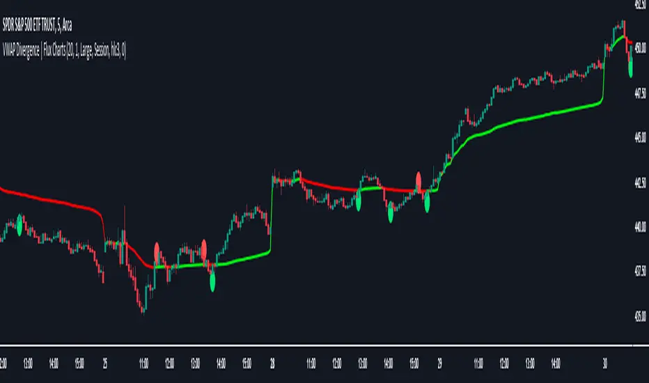
VWAP Divergence | Flux Charts The VWAP Divergence indicator aims to find divergences between price action and the VWAP indicator. It uses filters to filter out many of the false divergences and alert high quality, accurate signals. Red dots above the candle represent bearish divergences, while green dots below the candle represent bullish divergences. The main filter for divergences focuses on ATR and the price movement in the past candles up to the lookback period. Divergences are determined when a price movement over the lookback period is sharp enough to be greater/less than the ATR multiplier multiplied by the ATR. Settings Under "Divergence Settings", both the lookback period and ATR multiplier can be adjusted. Due to the nature of the calculations, the ATR multiplier and the lookback period should be set lower on higher time frames. As price movements become more averaged, for example on the 15 minute chart, sharp price movements happen less frequently and are often contained in fewer candles as they happen on lower time frames. Less volatile stocks such as KO, CL, or BAC should also use lower ATR multipliers and lower lookback periods. Under "Visual Settings", you can change the color of the VWAP line, show alternating VWAP colors, adjust divergence signal size, and show the VWAP line.

Flux Charts SFX Algo (Premium)Flux Charts SFX Algo indicator is a comprehensive and sophisticated all-in-one toolkit designed to cater to all the technical analysis needs of traders. Developed and designed by Russell W., head developer at Flux Charts. The Flux Charts SFX Algo indicator stands apart with its unique ability to seamlessly integrate with various forms of technical analysis, while also offering the option to function as a standalone toolkit adaptable to any trading style. The indicator has been designed to take into account the dynamic nature of market conditions, ensuring that every feature included remains relevant, reliable, and effective. Traders have countless possibilities when utilizing this indicator, allowing for the exploration and analysis of an array of cutting-edge features over time. This enables traders to selectively employ the features that align best with their individual trading styles and build a personal trading strategy. The Flux Charts SFX Algo indicator is set to revolutionize the way traders approach technical analysis, providing them with the tools and insights needed to navigate complex financial markets with confidence and precision. Flux Charts SFX Algo works in all markets (stocks, crypto, forex, futures, bonds, options, etc) and has many features including: Buy signals (Not to be followed blindly) Sell signals (Not to be followed blindly) Buy & Sell Signal Ratings (Higher rating doesn't necessarily mean a "better" signal) Algorithm Weighting Customization Algorithm Sensitivity Customization Algorithm Signal Strength Filter Take Profit signals Take Profit Retest signals Take Profit Level Optimization Trend Candle Coloring Volatility Bands + more What it does The indicator uses an Adjusted Weighted majority algorithm to generate "buy" and "sell" signals. The algorithm takes into account several market metrics and weights them based on their recent performance. How far back the algorithm checks is based on the “Time Weighting” setting. This allows users to choose between having more data points or having more recency bias within the algorithm, but less data to decipher. How it works and what differentiates it There are many popular strategies in the market all of which go in and out of successful periods. The SFX algorithm effectively uses popular indicators or "experts" and weights them using a period decided through the "Time Weighting" Setting. The "experts" include popular indicators that cover Momenutmn, ATR trends, and EMA trends. Adjusted Weighted Majority typically weighs only through binary events however the SFX also uses a dynamic system to punish larger losses. The total weighting is then used to confirm a signal is agreeing with the most successful "experts" or indicators within the time period. This effectively will filter poor signals during periods of underperformance compared to other indicators and the converse during performant periods. This weighting algorithm was inspired by the Princeton University lecture "Multiplicative Weight Algorithm" by Sanjeev Arora! Usage CME_MINI:ES1! 3 minute timeframe, July 7 2023. Indicator Settings: (Sensitivity: 70, Signal Strength: 40, Time Weighting: Recent Trends) The star-rated signals show the strength of the signals based on our weighting system The colored candles (green & red) simplify the market into basic uptrends/downtrends The volatility bands show areas of potential reversals The volatility bands also show potential breakouts (Tight bands = consolidation, which could lead to an impulsive move) The take profit signals suggest areas where profits should be taken in a trade Settings and their Usage Algorithm Settings Explained Sensitivity determines how frequently signals appear. A higher sensitivity would lead to more frequent signals (Buy & Sell) appearing on your chart Signal Strength helps filter out low-rated signals based on our Stochastic Weighting Algorithm. A higher signal strength will lead to fewer signals on your chart. A higher-rated signal doesn't necessarily make it a better signal than a lower-rated signal. Time Weighting allows you to choose how much historic data you want the indicator to use when interpreting data for the signals. There are three options to choose from including: - Recent Trends - Mixed Trends - Longterm Trends Using the "Recent Trends" option will only use recent market data when looking at the market metrics our algorithm uses for generating "Buy" and "Sell" signals. Thus, there will be a recency bias which means the metrics the algorithm is weighing more heavily have recently performed well. Using the "Longterm Trends" option will use more historic market data when looking at the market metrics our algorithm uses. This will give more data points for the algorithm to use, but it won't count for recent performances, but rather an overall performance in the past. Thus, if one metric has been doing poorly recently, it will still receive the same weight, even though it was performing well at the start of our lookback period for data. Using the "Mixed Trends" option will give you a choice that is in between these two options. This will give you a good balance between having enough data points for market metrics, while also sustaining a good bit of market recency bias.