Adaptive AI SuperTrend [AlgoPoint]🚀 Adaptive AI SuperTrend
Adaptive AI SuperTrend is a high-performance trading terminal that redefines trend-following by integrating Machine Learning (ML) principles with advanced market regime detection. Unlike static indicators, this system dynamically recalibrates its internal parameters to match the ever-changing volatility of the financial markets.
Equipped with a custom "Wizard Engine," it filters out market noise during consolidation and identifies high-probability trend continuation points, making it an essential tool for scalpers, day traders, and swing traders alike.
🧠 What Makes it "AI"?
While traditional indicators use fixed rules, Adaptive AI SuperTrend utilizes Algorithmic Intelligence to make real-time decisions:
KNN-Inspired Adaptation: The engine analyzes the last 150 bars of volatility and trend strength to automatically adjust its sensitivity.
Market Regime Intelligence: It distinguishes between "Trending" and "Ranging" states using a sophisticated Squeeze Momentum module, preventing "whipsaws" during low-volume periods.
Self-Backtesting Logic: The indicator continuously calculates its own historical Win-Rate. If the probability of success falls below a certain threshold, it suppresses lower-quality signals.
🛠 Key Features
Dynamic Consolidation Boxes: Automatically identifies and wraps "choppy" price action in professional gray boxes. It waits for 3+ bars of consolidation before marking the zone, helping you spot breakout opportunities early.
Multi-Strategy Aggression:
- Conservative: Filtered signals for long-term trend following.
- Balanced: Optimized for daily volatility.
- Aggressive: High-frequency signals for capturing micro-trends.
Dual-Exit Risk Management:
- ATR TP-SL Mode: Sets mathematical targets based on market volatility with persistent on-screen lines.
- Smart Trailing Mode: Rides the trend to its exhaustion point. Includes intelligent labeling (🎯 TP or 🛑 SL) based on the trade's net profitability.
- RSI Pullback Confirmation: Beyond simple trend flips, it detects "buy the dip" or "sell the rip" opportunities within an existing trend using RSI 50-level crossovers.
📊 Real-Time Analytics Dashboard
The integrated AlgoPoint Dashboard provides a surgical view of the market:
- Market State: Instant "Trending" vs. "Ranging" (Consolidation) detection.
- Trend Strength: ADX-based momentum tracking.
- Strategy Status: Real-time feedback on your active aggression and exit modes.
🎨 Clean Charting & Customization
Built for professional clarity, you have total control over the UI:
Toggle Consolidation Boxes on/off.
Toggle ATR Target Lines and Exit Labels.
Customize background filters and dashboard visibility.
Algotrading

BE-QuantFlow: Adaptive Momentum Trading█ Overview: QuantFlow: Adaptive Momentum Trading
QuantFlow is a sophisticated algorithmic momentum trading method designed specifically for indices and high-beta stocks. However, its logic is universal; with appropriate parameter tuning, it adapts to various asset classes and timeframes.
While the standard momentum indicators (like RSI or MACD) simply measure how fast price is moving (Velocity), QuantFlow analyzes the quality and conviction of the trend . Features like Dynamic Volatility Filtering and Trend Shielding, combined with volatility weighting and a "Dual-Line" approach to distinguish between a sustainable institutional trend and a temporary retail spike, make the indicator unique and more powerful.
█ Why QuantFlow ?
Quant (The Engine): This replaces subjective guessing with objective math.
Instead of just seeing that the price is "up," we measure "how it got there". For example, a stock that rises 1 currency value every day for 10 days (smooth trend) gets a much higher score than a stock that jumps 10 currency value in one minute and does nothing else (erratic noise). This mathematical rigor provides the structure.
█ Core Logic & Philosophy
To understand how QuantFlow calculates momentum, imagine a "Tug-of-War" between Buyers (Bulls) and Sellers (Bears). Most indicators (like RSI) use a single line. If RSI is at 50, it means "Neutral." But "Neutral" can mean two very different things:
Peace: Nothing is happening. No one is buying or selling.
War: Buyers are pushing hard, but Sellers are pushing back equally hard. Volatility is massive.
A single line hides this reality. QuantFlow splits the market into two separate scores:
Bull Score (Green Line): How hard are the buyers pushing?
Bear Score (Red Line): How hard are the sellers pushing?
The Layman's Advantage:
If both lines are low = Sleepy Market (Avoid).
If Green is high and Red is low = Clean Uptrend (Buy).
If Red is high and Green is low = Clean Downtrend (Sell).
If both lines are high = Chaos/War Zone (Wait).
█ How it Weight "Sustenance" (The Critical Quality Check)
This is the most unique aspect of QuantFlow: Trend direction alone is not enough; Sustenance is weighed equally . Standard indicators treat every 10 currency value movements the same way with no distinction. However, QuantFlow asks, "Did you hold the ground you gained?"
Scenario A (High Sustenance) : A stock opens at 100, marches to 110, and closes at 110.
Verdict : Buyers pushed up and sustained the price.
QuantFlow Weight : 100%. This is a high-quality move.
Scenario B (Low Sustenance) : A stock opens at 100, spikes to 110, but gets sold off to close at 102.
Verdict : Buyers pushed up (Trend is Up), but failed to sustain it (Long Wick).
QuantFlow Weight : 20%. This is treated as "Noise" or a trap.
By mathematically weighing the Close Location Value (where the candle closes relative to its high/low), QuantFlow filters out "Gap-and-Fade" traps and exhaustion spikes that fool traditional indicators.
Comparisons: QuantFlow vs. The Rest
Calculation Logic : Standard RSI/MACD measures simple price change over time. QuantFlow measures Price Change 'times (x)' Conviction (Sustenance Weighting).
Visual Output : Standard tools show a single line (0-100), often hiding market conflict. QuantFlow displays Dual Lines (Bull vs Bear Intensity) to reveal the true state of the battle.
Trap Handling : Standard indicators are often fooled by sharp spikes. QuantFlow ignores "Gap-and-Fade" moves with poor closing conviction.
Adaptability : Standard tools use static levels (e.g., Overbought > 70). QuantFlow uses Dynamic Bands that adjust automatically to recent volatility.
█ Dynamic Volatility Filtering
Unlike standard indicators that use fixed levels (e.g., "Buy if RSI > 50"), QuantFlow acknowledges that "50" means something different in a quiet market versus a crashing market. This section explains the statistical engine driving the signals.
The Problem with Static Levels : In a low-volatility environment, a momentum score of 55 might indicate a massive breakout. In a high-volatility environment, a score of 55 might just be random noise. A fixed threshold cannot handle both scenarios.
The Solution: Adaptive Statistics : The script maintains a memory of the Momentum Events. It doesn't just look at price; it looks at where the momentum occurred in the past and draws a "Noise Zone" (Grey Band). This logic acts as a "Smart Gatekeeper" for trade entries:
Scenario A: Inside the Noise (The Filter)
If a new momentum signal happens inside the Noise Zone, the script assumes it is likely chop or noise.
Action : It forces a wait period. The signal is delayed until the trend sustains itself for Confirm Bars; else the signal is cancelled. This filters out ~70% of false signals in sideways markets.
Scenario B: Outside the Noise (The Breakout)
If a new momentum signal happens outside the Noise Zone (or the momentum score smashes through the Upper Band), it is statistically significant (an outlier event).
Action: It triggers an Immediate Entry. No waiting is required because the move is powerful enough to escape the historical noise zone.
█ The ⚠️ "Warning" System (Heads-up for Smart Reversals)
While you are directional if there is potential reversal signal, it provides the heads-up warning for a better decision-making
█ Special Utility: Ghost Mode
For intraday traders, the biggest disruption to "Flow" is the mandatory broker square-off at 3:15 PM (considering Indian Market). Often, a trend continues overnight, and the trader misses the gap-up opening the next morning because their algo was flat.
Ghost Mode is a unique feature that runs silently in the background:
At Square-off: The strategy closes your official position to satisfy the broker.
In the Background: It keeps the trade "alive" virtually (Ghost).
Next Morning: If the market opens in the trend's favor, the strategy re-enters the trade automatically. This approach ensures you capture the full swing of the trend, even if you are forced to exit at the previous session.
█ Advice on this indicator:
Parameter Calibration: The default settings are optimized for BankNifty on 5-minute charts. If you trade stocks, crypto, commodities, or any higher timeframes (e.g., 15-min or hourly), you must adjust these.
Low Volatility Assets: Reduce Stop Multiplier to 2.0.
High Volatility Assets: Increase Momentum Lookback to 50 to filter noise.
Confluence (Additional Confirmation): While QuantFlow is a complete system, using it alongside Key Support/Resistance Levels or Volume Profile provides the highest probability setups.

Adaptive Bull Ratio Strategy█ Overview: Why This Strategy
Most option strategies fall into two traps:
They are too rigid: A "Call Ratio Spread" works great in slow markets but gets destroyed if the market rallies hard.
They are too simple: A simple "Buy Call" suffers from time decay (Theta) if the market chops sideways.
The Adaptive Bull Ratio Strategy solves both . It is a living strategy that "shifts gears" based on price action.
It is called "Adaptive" because it morphs its structure three times during a trade. It starts conservative to harvest Time Decay, but if the market explodes upwards, it "uncaps" itself to ride the trend aggressively.
█ The Entry Philosophy: Why Supertrend?
The default setting uses the Supertrend indicator as the trigger. This is intentional:
Volatility Awareness: Supertrend adapts to market noise using ATR. In high volatility, bands widen to prevent false entries.
Trend Confirmation: Since Phase 1 involves selling options, entering "too early" against a falling market is dangerous. Supertrend forces patience, waiting for a confirmed reversal (Close > Trend Line), ensuring the momentum is actually in your favor before you commit capital.
The "Drift" Benefit: This strategy excels in markets that "drift" upwards. Supertrend identifies these trends while filtering out short-term chop.
Flexibility with External Sources:
While Supertrend is the default, the strategy is designed to be flexible. You can enable the 'Enable External Source' option in the settings to plug in any custom indicator (e.g., Moving Averages, Parabolic SAR, or a proprietary trendline).
The Golden Rule for External Sources: The script interprets a Bullish Signal whenever your External Source line is below the Close price (Ext Source < Close).
Compatibility: As long as your custom indicator behaves like a support line in an uptrend (plotting below the candles), it will work seamlessly with this strategy's logic.
█ The "Long Only" Rationale: Avoiding the Volatility Trap
Why not trade this on the short side (Puts) during crashes?
The Volatility Trap (Vega Risk): In Bull markets, Implied Volatility (IV) usually drops, helping your sold options decay faster. In Bear markets, IV explodes (panic). Selling OTM Puts during a crash is dangerous as their value skyrockets, neutralizing gains.
Velocity Risk: Bear markets crash fast ("Elevator Down"). Prices can blow through adjustment levels faster than the strategy can safely roll down, causing slippage.
Structural Skew: OTM Puts are inherently more expensive. Buying expensive ITM Puts and selling expensive OTM Puts shifts the breakeven further away, making V-shape recoveries painful.
█ How It Works & Stands Out
This strategy actively transforms risk profiles based on market movement:
Phase 1: The "Safe" Start (Entry)
Setup: Initiates a Call Ratio Spread (Buy 2 ITM, Sell 4 OTM) + Protective Puts.
Logic: Profits from sideways drift or slow rallies via Time Decay (Theta). The sold options finance the trade.
Phase 2: The "Shift" (Adjustment Level 1)
Trigger: Market moves above Leg 2 (3 OTM Call).
Action: Rolls Up the position. Exits initial legs, enters new higher legs, and adds a Short Put to finance the roll.
Impact: Aggressive. You bet the trend is strong enough to support the added downside risk of the short put.
Phase 3: The "Uncap" (Adjustment Level 2)
Trigger: Market moves above Leg 3 (4 OTM Call).
Action: Exits all Sold Calls.
Impact: Uncaps profit potential. The trade becomes a Net Long position (Long Calls + Short Puts), allowing you to ride a massive rally without a ceiling.
Phase 4: The "Lock-In" (Optional Trail Adjustment)
Trigger: The market goes parabolic (price rises X levels above Leg 3, configurable in settings).
Action (If Enabled):
Call Adj: Exits the Phase 3 calls and buys fresh 1-OTM calls (Rolling Up to lock profits).
Put Adj: Exits all Put legs (Removing downside risk completely).
Impact: Maximum Safety. This phase is about "banking" the windfall from a massive rally and leaving a smaller, risk-free runner to capture any final extension.
█ How to Start: A Quick Setup Guide
Step 1: Map Expiry Dates
Manually input your trading expiry dates in Settings -> Expiry Management.
Format: YYYY-MM-DD (e.g., 2025-12-25). Strict adherence required for DhanHQ.
Step 2: Configure Symbol & Size
Exchange/Symbol: Enter NSE and NIFTY (or your ticker).
Lot Multiplier: Default is 1. Set to 2 to double all quantities (e.g., Buy 2 becomes Buy 4).
Step 3: Understand Visuals
Entry Window (Light Blue): Strategy is scanning for new trades.
Non-Entry Window (Dark Blue): Trading blocked (Day before Expiry & Expiry Day). Only management allowed.
Green Box: Valid Late Entry Zone.
Red Dashed Line: Invalidation Level (if price touches this, no late entry).
Fuchsia Line: Trigger level for Special Trail Adjustments (Phase 4).
IMPORTANT: Broker & Technology Heads-Up:
The alerts generated by this script ({"secret": "...", "alertType": "multi_leg_order"...}) are specifically formatted for the DhanHQ webhook structure.
Dhan Users: Plug-and-play.
Other Brokers: You need middleware (NextLevelBot, Quantiply) to parse the JSON.
█ Risk Disclaimer & Advice
Trading options involves substantial risk.
The Whipsaw Risk: In Phase 2, you are Long Calls and Short Puts. A sharp reversal causes losses on both sides.
Margin: Selling options requires significant margin. Keep a 15-20% cash buffer to handle adjustments instantly.
Testing: This strategy is optimized for NIFTY Weekly Options. Effectiveness on BankNifty or Stocks is untested and may require parameter tuning.
Advice:
Backtest: Use TradingView Replay.
Paper Trade: Run for at least one expiry cycle before live deployment.
Consult: Seek professional financial advice before trading.
Practical Tips for Smooth Execution
For a new trader deploying this system, these operational tips are vital:
Capital Buffer: Do not trade at your limit. Always keep 10-15% free cash in your broker account. Adjustments (specifically Phase 2, where you sell an extra Put) require additional margin instantly. If margin is short, the order fails, and your hedge breaks.
Liquidity Awareness : The script trades "Far Deep OTM" options (Leg 4) to reduce margin. On indices like Nifty/BankNifty, this is fine. On individual stocks, these deep strikes might be illiquid. Check the option chain volume before deploying on stocks.
Trust the Process (but Verify) : While the algo drives, you are the pilot.
Check your API connection every morning.
Ensure the "Entry Window" background color on the chart matches your real-world date.
Verify that your broker executed all legs of a multi-leg order (partial fills are rare but possible).
The "Human" Stop: If major news breaks (e.g., unexpected election results, war announcements), volatility can expand faster than any algo can react. It is acceptable—and smart—to pause the strategy during known "Black Swan" events or earnings releases.
█ Timeframe Selection: The 30-Minute Standard
Critical Requirement: This indicator must be applied to a 30-minute chart.
Why?
Noise Filtering: The Supertrend logic is tuned to capture multi-day trends. Lower timeframes (5m, 15m) are full of "noise"—random fluctuations that look like trend changes but aren't.
Execution Logic (The Hybrid Engine): The script has a built-in "Dual Timeframe" architecture.
Decision Layer (30m): Uses the chart timeframe to decide when to be Bullish or Bearish.
Execution Layer (5m): Internally fetches 5-minute data to manage the how (Adjustments, Late Entries, and precise invalidation).
The Risk of Lower Timeframes: If you run the main chart on 5-minutes, you destroy this hierarchy. You will get too many signals, pay too much brokerage, and the internal logic may behave erratically.
Recommendation: Always keep your TradingView chart interval at 30m. Do not switch to lower timeframes expecting "faster" signals; you will likely just get "false" signals.
█ Testing Scope, Feedback
⚠️ Important Note on Asset Classes:
This strategy logic and the associated strike step calculations have been rigorously tested ONLY on NIFTY Index Options with Weekly Expiry.
BankNifty / Sensex / FinNifty: The volatility characteristics (ATR) and strike intervals of these instruments differ significantly from NIFTY. The effectiveness of this strategy on these other scripts has not been verified and may require different parameter tuning (e.g., strike_step or ATR Length).
Stocks: Individual stock options often lack the liquidity required for the "Deep OTM" legs, leading to potential execution failures.
We encourage traders to backtest this logic on other indices and share their findings! If you find a robust parameter set for BankNifty or observe unique behaviors on other scripts, please let us know in the comments below so we can improve the algorithm for everyone. Your feedback is appriciated.

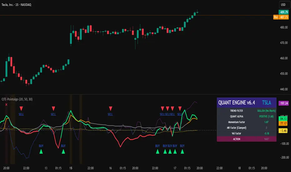
QUANT TRADING ENGINE [PointAlgo]Quant Trading Engine is a quantitative market-analysis indicator that combines multiple statistical factors to study trend behavior, mean reversion, volatility, execution efficiency, and market stability.
The indicator converts raw price behavior into standardized signals to help evaluate directional bias and risk conditions in a systematic way.
This script focuses on factor alignment and regime awareness, not prediction certainty.
Design Philosophy
Markets move through different regimes such as trending, ranging, volatile expansion, and instability.
This indicator attempts to model these regimes by blending:
Momentum strength
Mean-reversion pressure
Volatility risk
Trend filtering
Execution context (VWAP)
Correlation structure
Each component is normalized and combined into a single Quant Alpha framework.
Factor Construction
1. Momentum Factor
Measures directional strength using percentage price change over a rolling window.
Standardized using mean and standard deviation.
Represents trend continuation pressure.
2. Mean Reversion Factor
Measures deviation from a longer moving average.
Standardized to identify stretched conditions.
Designed to capture counter-trend behavior.
Directional Clamping
Mean-reversion signals are dynamically restricted:
No counter-trend buying during downtrends.
No counter-trend selling during uptrends.
Allows both sides only in neutral regimes.
This prevents conflicting signals in strong trends.
3. Volatility Factor
Uses realized volatility derived from price changes.
Penalizes environments where volatility deviates significantly from its norm.
Acts as a risk adjustment rather than a directional driver.
4. Composite Quant Alpha
The final Quant Alpha is a weighted blend of:
Momentum
Mean reversion (trend-clamped)
Volatility risk
The composite is standardized into a Z-score, allowing consistent interpretation across instruments and timeframes.
Signal Logic
Buy signal occurs when Quant Alpha crosses above zero.
Sell signal occurs when Quant Alpha crosses below zero.
Zero-cross logic is used to represent shifts from negative to positive statistical bias and vice versa.
Signals reflect statistical regime change, not trade instructions.
Volatility Smile Context
Measures price deviation from its statistical distribution.
Identifies skewed conditions where upside or downside volatility becomes dominant.
Highlights extreme deviations that may imply elevated derivative risk.
Exotic Risk Conditions
Detects sudden price expansion combined with volatility spikes.
Highlights environments where execution and risk become unstable.
Visual background cues are used for awareness only.
Execution Context (VWAP)
Measures price distance from VWAP.
Used to assess execution efficiency rather than direction.
Helps identify stretched conditions relative to average traded price.
Correlation Structure
Evaluates short-term return correlations.
Detects when price behavior becomes less predictable.
Flags structural instability rather than trend direction.
Visualization
The indicator plots:
Quant Alpha (scaled) with directional coloring
Volatility smile deviation
Price vs VWAP distance
Correlation structure
Signal markers indicate Quant Alpha zero-cross events and risk conditions.
Dashboard
A compact dashboard summarizes:
Trend filter state
Quant Alpha polarity and value
Individual factor readings
Current action state (Buy / Sell / Wait / Risk)
The dashboard provides a real-time snapshot of internal model conditions.
Usage Notes
Designed for analytical interpretation and research.
Best used alongside price action and risk management tools.
Factor behavior depends on instrument liquidity and volatility.
Not optimized for illiquid or irregular markets.
Disclaimer
This script is provided for educational and analytical purposes only.
It does not provide financial, investment, or trading advice.
All outputs should be independently validated before making any trading decisions.
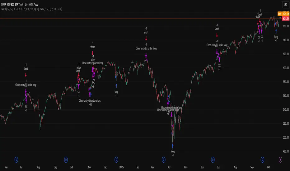
Mutanabby_AI | ONEUSDT_MR1
ONEUSDT Mean-Reversion Strategy | 74.68% Win Rate | 417% Net Profit
This is a long-only mean-reversion strategy designed specifically for ONEUSDT on the 1-hour timeframe. The core logic identifies oversold conditions following sharp declines and enters positions when selling pressure exhausts, capturing the subsequent recovery bounce.
Backtested Period: June 2019 – December 2025 (~6 years)
Performance Summary
| Metric | Value |
|--------|-------|
| Net Profit | +417.68% |
| Win Rate | 74.68% |
| Profit Factor | 4.019 |
| Total Trades | 237 |
| Sharpe Ratio | 0.364 |
| Sortino Ratio | 1.917 |
| Max Drawdown | 51.08% |
| Avg Win | +3.14% |
| Avg Loss | -2.30% |
| Buy & Hold Return | -80.44% |
Strategy Logic :
Entry Conditions (Long Only):
The strategy seeks confluence of three conditions that identify exhausted selling:
1. Prior Move Filter:*The price change from 5 bars ago to 3 bars ago must be ≥ -7% (ensures we're not entering during freefall)
2. Current Move Filter: The price change over the last 2 bars must be ≤ 0% (confirms momentum is stalling or reversing)
3. Three-Bar Decline: The price change from 5 bars ago to 3 bars ago must be ≤ -5% (confirms a significant recent drop occurred)
When all three conditions align, the strategy identifies a potential reversal point where sellers are exhausted.
Exit Conditions:
- Primary Exit: Close above the previous bar's high while the open of the previous bar is at or below the close from 9 bars ago (profit-taking on strength)
- Trailing Stop: 11x ATR trailing stop that locks in profits as price rises
Risk Management
- Position Sizing:Fixed position based on account equity divided by entry price
- Trailing Stop:11× ATR (14-period) provides wide enough room for crypto volatility while protecting gains
- Pyramiding:Up to 4 orders allowed (can scale into winning positions)
- **Commission:** 0.1% per trade (realistic exchange fees included)
Important Disclaimers
⚠️ This is NOT financial advice.
- Past performance does not guarantee future results
- Backtest results may contain look-ahead bias or curve-fitting
- Real trading involves slippage, liquidity issues, and execution delays
- This strategy is optimized for ONEUSDT specifically — results may differ on other pairs
- Always test before risking real capital
Recommended Usage
- Timeframe:*1H (as designed)
- Pair: ONEUSDT (Binance)
- Account Size: Ensure sufficient capital to survive max drawdown
Source Code
Feedback Welcome
I'm sharing this strategy freely for educational purposes. Please:
- Drop a comment with your backtesting results any you analysis
- Share any modifications that improve performance
- Let me know if you spot any issues in the logic
Happy trading
As a quant trader, do you think this strategy will survive in live trading?
Yes or No? And why?
I want to hear from you guys

Smart Cloud by Ilker (Custom Matriks)A Proprietary Hybrid Trend System for All Major Financial Assets
This indicator, originally developed for the Matriks platform, is a highly effective hybrid trend identification system designed for day-to-day analysis across all major asset classes, including Stocks, Forex, Indices, and Cryptocurrencies. It combines the forward-looking principle of the Ichimoku Kinko Hyo Cloud with heavily smoothed Moving Averages (MAs) to create a clear, visually guided trading signal. (Daily Timeframe recommended for optimal results).
📊 Algorithmic Structure and Parameters
The "Smart Cloud" utilizes six primary user-adjustable parameters that govern its sensitivity and shape, moving away from standard Ichimoku settings to provide a robust, customized trend view:
P1, P2, P3 (60, 56, 248): These long-term settings define the core structure and width of the cloud, acting as the primary dynamic support and resistance zone. The significantly longer P3 (Lagging Period) ensures the cloud reflects strong, deep market cycles.
P4 (Displacement 26): Maintains the traditional Ichimoku principle of projecting the cloud 26 periods forward to provide a predictive view of future trend support/resistance.
P5 (MA50 - Blue) & P6 (MA10 - Purple): These are the two primary Moving Averages plotted inside the cloud. They serve as fast-response momentum lines:
P5 (MA50): Represents the middle-term trend average.
P6 (MA10): Represents the short-term market momentum.
📈 Core Trend and Signal Interpretation
The indicator provides powerful trend identification based on three key components:
The Cloud (Kumo):
Green Cloud (Bullish): Indicates the dominant trend is up, suggesting dynamic support for price action.
Red Cloud (Bearish): Indicates the dominant trend is down, suggesting dynamic resistance.
The thickness and slope of the cloud are key indicators of trend strength.
MA Crossover Signal (Blue/Purple):
Buy Signal: When the faster Purple MA (P6=10) crosses above the slower Blue MA (P5=50).
Sell Signal: When the faster Purple MA (P6=10) crosses below the slower Blue MA (P5=50).
Price Action & Confirmation:
The most powerful signals occur when a MA Crossover is confirmed by price breaking out of the cloud in the same direction.
Price above the cloud and MA crossover to the upside suggests a strong buy entry.
Disclaimer: This tool is intended for analysis and decision-making support. It is not financial advice. Always use stop-loss orders and manage your risk accordingly.

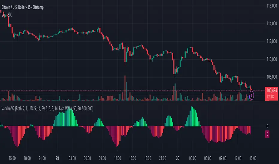
Vandan V2Vandan V2 is an automated trend-following strategy for NASDAQ E-mini Futures (NQ1!).
It uses multi-timeframe momentum and volatility filters to identify high-probability entries.
Includes dynamic risk management and trailing logic optimized for intraday trading.
DayFlow VWAP Relay Forex Majors StrategySummary in one paragraph
DayFlow VWAP Relay is a day-trading strategy for major FX pairs on intraday timeframes, demonstrated on EURUSD 15 minutes. It waits for alignment between a daily anchored VWAP regime check, residual percentiles, and lower-timeframe micro flow before suggesting trades. The originality is the fusion of daily VWAP residual percentiles with a live micro-flow score from 1 minute data to switch between fade and breakout behavior inside the same session. Add it to a clean chart and use the markers and alerts.
Scope and intent
• Markets: Major FX pairs such as EURUSD, GBPUSD, USDJPY, AUDUSD, USDCHF, USDCAD
• Timeframes: One minute to one hour
• Default demo in this publication: EURUSD on 15 minutes
• Purpose: Reduce false starts by acting only when context, location and micro flow agree
• Limits: This is a strategy. Orders are simulated on standard candles only
Originality and usefulness
• Core novelty: Residual percentiles to daily anchored VWAP decide “balanced versus expanding day”. A separate 1 minute micro-flow score confirms direction, so the same model fades extremes in balance and rides range breaks in expansion
• Failure modes addressed: Chop fakeouts and unconfirmed breakouts are filtered by the expansion gate and micro-flow threshold
• Testability: Every input is exposed. Bands, background regime color, and markers show why a suggestion appears
• Portable yardstick: Stops and targets are ATR multiples converted to ticks, which transfer across symbols
• Open source status: No reused third-party code that requires attribution
Method overview in plain language
The day is anchored with a VWAP that updates from the daily session start. Price minus VWAP is the residual. Percentiles of that residual measured over a rolling window define location extremes for the current day. A regime score compares residual volatility to price volatility. When expansion is low, the day is treated as balanced and the model fades residual extremes if 1 minute micro flow points back to VWAP. When expansion is high, the model trades breakouts outside the VWAP bands if slope and micro flow agree with the move.
Base measures
• Range basis: True Range smoothed by ATR for stops and targets, length 14
• Return basis: Not required for signals; residuals are absolute price distance to VWAP
Components
• Daily Anchor VWAP Bands. VWAP with standard-deviation bands. Slope sign is used for trend confirmation on breakouts
• Residual Percentiles. Rolling percentiles of close minus VWAP over Signal length. Identify location extremes inside the day
• Expansion Ratio. Standard deviation of residuals divided by standard deviation of price over Signal length. Classifies balanced versus expanding day
• Micro Flow. Net up minus down closes from 1 minute data across a short span, normalized to −1..+1. Confirms direction and avoids fades against pressure
• Session Window optional. Restricts trading to your configured hours to avoid thin periods
• Cooldown optional. Bars to wait after a position closes to prevent immediate re-entry
Fusion rule
Gating rather than weighting. First choose regime by Expansion Ratio versus the Expansion gate. Inside each regime all listed conditions must be true: location test plus micro-flow threshold plus session window plus cooldown. Breakouts also require VWAP slope alignment.
Signal rule
• Long suggestion on balanced day: residual at or below the lower percentile and micro flow positive above the gate while inside session and cooldown is satisfied
• Short suggestion on balanced day: residual at or above the upper percentile and micro flow negative below the gate while inside session and cooldown is satisfied
• Long suggestion on expanding day: close above the upper VWAP band, VWAP slope positive, micro flow positive, session and cooldown satisfied
• Short suggestion on expanding day: close below the lower VWAP band, VWAP slope negative, micro flow negative, session and cooldown satisfied
• Positions flip on opposite suggestions or exit by brackets
What you will see on the chart
• Markers on suggestion bars: L for long, S for short
• Exit occurs on reverse signal or when a bracket order is filled
• Reference lines: daily anchored VWAP with upper and lower bands
• Optional background: teal for balanced day, orange for expanding day
Inputs with guidance
Setup
• Signal length. Residual and regime window. Typical 40 to 100. Higher smooths, lower reacts faster
Micro Flow
• Micro TF. Lower timeframe used for micro flow, default 1 minute
• Micro span bars. Count of lower-TF bars. Typical 5 to 20
• Micro flow gate 0..1. Minimum absolute flow. Raising it demands stronger confirmation and reduces trade count
VWAP Bands
• VWAP stdev multiplier. Band width. Typical 0.8 to 1.6. Wider bands reduce breakout frequency and increase fade distance
• Expansion gate 0..3. Threshold to switch from fades to breakouts. Raising it favors fades, lowering it favors breakouts
Sessions
• Use session filter. Enable to trade only inside your window
• Trade window UTC. Default 07:00 to 17:00
Risk
• ATR length. Stop and target basis. Typical 10 to 21
• Stop ATR x. Initial stop distance in ATR multiples
• Target ATR x. Profit target distance in ATR multiples
• Cooldown bars after close. Wait bars before a new entry
• Side. Both, long only, or short only
View
• Show VWAP and bands
• Color bars by residual regime
Properties visible in this publication
• Initial capital 10000
• Base currency Default
• request.security uses lookahead off everywhere
• Strategy: Percent of equity with value 3. Pyramiding 0. Commission cash per order 0.0001 USD. Slippage 3 ticks. Process orders on close ON. Bar magnifier ON. Recalculate after order is filled OFF. Calc on every tick OFF. Using standard OHLC fills ON.
Realism and responsible publication
No performance claims. Past results never guarantee future outcomes. Fills and slippage vary by venue. Shapes can move while a bar forms and settle on close. Strategies must run on standard candles for signals and orders.
Honest limitations and failure modes
High impact news, session opens, and thin liquidity can invalidate assumptions. Very quiet days can reduce contrast between residuals and price volatility. Session windows use the chart exchange time. If both stop and target are touched within a single bar, TradingView’s standard OHLC price-movement model decides the outcome.
Expect different behavior on illiquid pairs or during holidays. The model is sensitive to session definitions and feed time. Past results never guarantee future outcomes.
Legal
Education and research only. Not investment advice. You are responsible for your decisions. Test on historical data and in simulation before any live use. Use realistic costs.

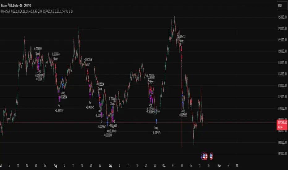
Hyper SAR Reactor Trend StrategyHyperSAR Reactor Adaptive PSAR Strategy
Summary
Adaptive Parabolic SAR strategy for liquid stocks, ETFs, futures, and crypto across intraday to daily timeframes. It acts only when an adaptive trail flips and confirmation gates agree. Originality comes from a logistic boost of the SAR acceleration using drift versus ATR, plus ATR hysteresis, inertia on the trail, and a bear-only gate for shorts. Add to a clean chart and run on bar close for conservative alerts.
Scope and intent
• Markets: large cap equities and ETFs, index futures, major FX, liquid crypto
• Timeframes: one minute to daily
• Default demo: BTC on 60 minute
• Purpose: faster yet calmer PSAR that resists chop and improves short discipline
• Limits: this is a strategy that places simulated orders on standard candles
Originality and usefulness
• Novel fusion: PSAR AF is boosted by a logistic function of normalized drift, trail is monotone with inertia, entries use ATR buffers and optional cooldown, shorts are allowed only in a bear bias
• Addresses false flips in low volatility and weak downtrends
• All controls are exposed in Inputs for testability
• Yardstick: ATR normalizes drift so settings port across symbols
• Open source. No links. No solicitation
Method overview
Components
• Adaptive AF: base step plus boost factor times logistic strength
• Trail inertia: one sided blend that keeps the SAR monotone
• Flip hysteresis: price must clear SAR by a buffer times ATR
• Volatility gate: ATR over its mean must exceed a ratio
• Bear bias for shorts: price below EMA of length 91 with negative slope window 54
• Cooldown bars optional after any entry
• Visual SAR smoothing is cosmetic and does not drive orders
Fusion rule
Entry requires the internal flip plus all enabled gates. No weighted scores.
Signal rule
• Long when trend flips up and close is above SAR plus buffer times ATR and gates pass
• Short when trend flips down and close is below SAR minus buffer times ATR and gates pass
• Exit uses SAR as stop and optional ATR take profit per side
Inputs with guidance
Reactor Engine
• Start AF 0.02. Lower slows new trends. Higher reacts quicker
• Max AF 1. Typical 0.2 to 1. Caps acceleration
• Base step 0.04. Typical 0.01 to 0.08. Raises speed in trends
• Strength window 18. Typical 10 to 40. Drift estimation window
• ATR length 16. Typical 10 to 30. Volatility unit
• Strength gain 4.5. Typical 2 to 6. Steepness of logistic
• Strength center 0.45. Typical 0.3 to 0.8. Midpoint of logistic
• Boost factor 0.03. Typical 0.01 to 0.08. Adds to step when strength rises
• AF smoothing 0.50. Typical 0.2 to 0.7. Adds inertia to AF growth
• Trail smoothing 0.35. Typical 0.15 to 0.45. Adds inertia to the trail
• Allow Long, Allow Short toggles
Trade Filters
• Flip confirm buffer ATR 0.50. Typical 0.2 to 0.8. Raise to cut flips
• Cooldown bars after entry 0. Typical 0 to 8. Blocks re entry for N bars
• Vol gate length 30 and Vol gate ratio 1. Raise ratio to trade only in active regimes
• Gate shorts by bear regime ON. Bear bias window 54 and Bias MA length 91 tune strictness
Risk
• TP long ATR 1.0. Set to zero to disable
• TP short ATR 0.0. Set to 0.8 to 1.2 for quicker shorts
Usage recipes
Intraday trend focus
Confirm buffer 0.35 to 0.5. Cooldown 2 to 4. Vol gate ratio 1.1. Shorts gated by bear regime.
Intraday mean reversion focus
Confirm buffer 0.6 to 0.8. Cooldown 4 to 6. Lower boost factor. Leave shorts gated.
Swing continuation
Strength window 24 to 34. ATR length 20 to 30. Confirm buffer 0.4 to 0.6. Use daily or four hour charts.
Properties visible in this publication
Initial capital 10000. Base currency USD. Order size Percent of equity 3. Pyramiding 0. Commission 0.05 percent. Slippage 5 ticks. Process orders on close OFF. Bar magnifier OFF. Recalculate after order filled OFF. Calc on every tick OFF. No security calls.
Realism and responsible publication
No performance claims. Past results never guarantee future outcomes. Shapes can move while a bar forms and settle on close. Strategies execute only on standard candles.
Honest limitations and failure modes
High impact events and thin books can void assumptions. Gap heavy symbols may prefer longer ATR. Very quiet regimes can reduce contrast and invite false flips.
Open source reuse and credits
Public domain building blocks used: PSAR concept and ATR. Implementation and fusion are original. No borrowed code from other authors.
Strategy notice
Orders are simulated on standard candles. No lookahead.
Entries and exits
Long: flip up plus ATR buffer and all gates true
Short: flip down plus ATR buffer and gates true with bear bias when enabled
Exit: SAR stop per side, optional ATR take profit, optional cooldown after entry
Tie handling: stop first if both stop and target could fill in one bar
TriAnchor Elastic Reversion US Market SPY and QQQ adaptedSummary in one paragraph
Mean-reversion strategy for liquid ETFs, index futures, large-cap equities, and major crypto on intraday to daily timeframes. It waits for three anchored VWAP stretches to become statistically extreme, aligns with bar-shape and breadth, and fades the move. Originality comes from fusing daily, weekly, and monthly AVWAP distances into a single ATR-normalized energy percentile, then gating with a robust Z-score and a session-safe gap filter.
Scope and intent
• Markets: SPY QQQ IWM NDX large caps liquid futures liquid crypto
• Timeframes: 5 min to 1 day
• Default demo: SPY on 60 min
• Purpose: fade stretched moves only when multi-anchor context and breadth agree
• Limits: strategy uses standard candles for signals and orders only
Originality and usefulness
• Unique fusion: tri-anchor AVWAP energy percentile plus robust Z of close plus shape-in-range gate plus breadth Z of SPY QQQ IWM
• Failure mode addressed: chasing extended moves and fading during index-wide thrusts
• Testability: each component is an input and visible in orders list via L and S tags
• Portable yardstick: distances are ATR-normalized so thresholds transfer across symbols
• Open source: method and implementation are disclosed for community review
Method overview in plain language
Base measures
• Range basis: ATR(length = atr_len) as the normalization unit
• Return basis: not used directly; we use rank statistics for stability
Components
• Tri-Anchor Energy: squared distances of price from daily, weekly, monthly AVWAPs, each divided by ATR, then summed and ranked to a percentile over base_len
• Robust Z of Close: median and MAD based Z to avoid outliers
• Shape Gate: position of close inside bar range to require capitulation for longs and exhaustion for shorts
• Breadth Gate: average robust Z of SPY QQQ IWM to avoid fading when the tape is one-sided
• Gap Shock: skip signals after large session gaps
Fusion rule
• All required gates must be true: Energy ≥ energy_trig_prc, |Robust Z| ≥ z_trig, Shape satisfied, Breadth confirmed, Gap filter clear
Signal rule
• Long: energy extreme, Z negative beyond threshold, close near bar low, breadth Z ≤ −breadth_z_ok
• Short: energy extreme, Z positive beyond threshold, close near bar high, breadth Z ≥ +breadth_z_ok
What you will see on the chart
• Standard strategy arrows for entries and exits
• Optional short-side brackets: ATR stop and ATR take profit if enabled
Inputs with guidance
Setup
• Base length: window for percentile ranks and medians. Typical 40 to 80. Longer smooths, shorter reacts.
• ATR length: normalization unit. Typical 10 to 20. Higher reduces noise.
• VWAP band stdev: volatility bands for anchors. Typical 2.0 to 4.0.
• Robust Z window: 40 to 100. Larger for stability.
• Robust Z entry magnitude: 1.2 to 2.2. Higher means stronger extremes only.
• Energy percentile trigger: 90 to 99.5. Higher limits signals to rare stretches.
• Bar close in range gate long: 0.05 to 0.25. Larger requires deeper capitulation for longs.
Regime and Breadth
• Use breadth gate: on when trading indices or broad ETFs.
• Breadth Z confirm magnitude: 0.8 to 1.8. Higher avoids fighting thrusts.
• Gap shock percent: 1.0 to 5.0. Larger allows more gaps to trade.
Risk — Short only
• Enable short SL TP: on to bracket shorts.
• Short ATR stop mult: 1.0 to 3.0.
• Short ATR take profit mult: 1.0 to 6.0.
Properties visible in this publication
• Initial capital: 25000USD
• Default order size: Percent of total equity 3%
• Pyramiding: 0
• Commission: 0.03 percent
• Slippage: 5 ticks
• Process orders on close: OFF
• Bar magnifier: OFF
• Recalculate after order is filled: OFF
• Calc on every tick: OFF
• request.security lookahead off where used
Realism and responsible publication
• No performance claims. Past results never guarantee future outcomes
• Fills and slippage vary by venue
• Shapes can move during bar formation and settle on close
• Standard candles only for strategies
Honest limitations and failure modes
• Economic releases or very thin liquidity can overwhelm mean-reversion logic
• Heavy gap regimes may require larger gap filter or TR-based tuning
• Very quiet regimes reduce signal contrast; extend windows or raise thresholds
Open source reuse and credits
• None
Strategy notice
Orders are simulated by TradingView on standard candles. request.security uses lookahead off where applicable. Non-standard charts are not supported for execution.
Entries and exits
• Entry logic: as in Signal rule above
• Exit logic: short side optional ATR stop and ATR take profit via brackets; long side closes on opposite setup
• Risk model: ATR-based brackets on shorts when enabled
• Tie handling: stop first when both could be touched inside one bar
Dataset and sample size
• Test across your visible history. For robust inference prefer 100 plus trades.
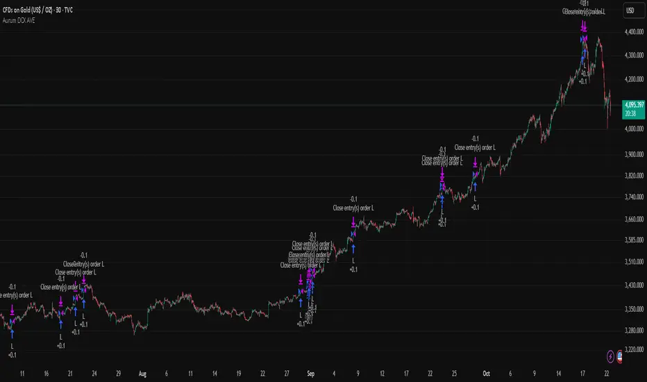
Aurum DCX AVE Gold and Silver StrategySummary in one paragraph
Aurum DCX AVE is a volatility break strategy for gold and silver on intraday and swing timeframes. It aligns a new Directional Convexity Index with an Adaptive Volatility Envelope and an optional USD/DXY bias so trades appear only when direction quality and expansion agree. It is original because it fuses three pieces rarely combined in one model for metals: a convexity aware trend strength score, a percentile based envelope that widens with regime heat, and an intermarket DXY filter.
Scope and intent
• Markets. Gold and silver futures or spot, other liquid commodities, major indices
• Timeframes. Five minutes to one day. Defaults to 30min for swing pace
• Default demo used in this publication. TVC:GOLD on 30m
• Purpose. Enter confirmed volatility breaks while muting chop using regime heat and USD bias
• Limits. This is a strategy. Orders are simulated on standard candles only
Originality and usefulness
• Unique fusion. DCX combines DI strength with path efficiency and curvature. AVE blends ATR with a high TR percentile and widens with DCX heat. DXY adds an intermarket bias
• Failure mode addressed. False starts inside compression and unconfirmed breakouts during USD swings
• Testability. Each component has a named input. Entry names L and S are visible in the list of trades
• Portable yardstick. Weekly ATR for stops and R multiples for targets
• Open source. Method and implementation are disclosed for community review
Method overview in plain language
You score direction quality with DCX, size an adaptive envelope with a blend of ATR and a high TR percentile, and only allow breaks that clear the band while DCX is above a heat threshold in the same direction. An optional DXY filter favors long when USD weakens and short when USD strengthens. Orders are bracketed with a Weekly ATR stop and an R multiple target, with optional trailing to the envelope.
Base measures
• Range basis. True Range and ATR over user windows. A high TR percentile captures expansion tails used by AVE
• Return basis. Not required
Components
• Directional Convexity Index DCX. Measures directional strength with DX, multiplies by path efficiency, blends a curvature term from acceleration, scales to 0 to 100, and uses a rise window
• Adaptive Volatility Envelope AVE. Midline ALMA or HMA or EMA plus bands sized by a blend of ATR and a high TR percentile. The blend weight follows volatility of volatility. Band width widens with DCX heat
• DXY Bias optional. Daily EMA trend of DXY. Long bias when USD weakens. Short bias when USD strengthens
• Risk block. Initial stop equals Weekly ATR times a multiplier. Target equals an R multiple of the initial risk. Optional trailing to AVE band
Fusion rule
• All gates must pass. DCX above threshold and rising. Directional lead agrees. Price breaks the AVE band in the same direction. DXY bias agrees when enabled
Signal rule
• Long. Close above AVE upper and DCX above threshold and DCX rising and plus DI leads and DXY bias is bearish
• Short. Close below AVE lower and DCX above threshold and DCX falling and minus DI leads and DXY bias is bullish
• Exit and flip. Bracket exit at stop or target. Optional trailing to AVE band
Inputs with guidance
Setup
• Symbol. Default TVC:GOLD (Correlation Asset for internal logic)
• Signal timeframe. Blank follows the chart
• Confirm timeframe. Default 1 day used by the bias block
Directional Convexity Index
• DCX window. Typical 10 to 21. Higher filters more. Lower reacts earlier
• DCX rise bars. Typical 3 to 6. Higher demands continuation
• DCX entry threshold. Typical 15 to 35. Higher avoids soft moves
• Efficiency floor. Typical 0.02 to 0.06. Stability in quiet tape
• Convexity weight 0..1. Typical 0.25 to 0.50. Higher gives curvature more influence
Adaptive Volatility Envelope
• AVE window. Typical 24 to 48. Higher smooths more
• Midline type. ALMA or HMA or EMA per preference
• TR percentile 0..100. Typical 75 to 90. Higher favors only strong expansions
• Vol of vol reference. Typical 0.05 to 0.30. Controls how much the percentile term weighs against ATR
• Base envelope mult. Typical 1.4 to 2.2. Width of bands
• Regime adapt 0..1. Typical 0.6 to 0.95. How much DCX heat widens or narrows the bands
Intermarket Bias
• Use DXY bias. Default ON
• DXY timeframe. Default 1 day
• DXY trend window. Typical 10 to 50
Risk
• Risk percent per trade. Reporting field. Keep live risk near one to two percent
• Weekly ATR. Default 14. Basis for stops
• Stop ATR weekly mult. Typical 1.5 to 3.0
• Take profit R multiple. Typical 1.5 to 3.0
• Trail with AVE band. Optional. OFF by default
Properties visible in this publication
• Initial capital. 20000
• Base currency. USD
• request.security lookahead off everywhere
• Commission. 0.03 percent
• Slippage. 5 ticks
• Default order size method percent of equity with value 3% of the total capital available
• Pyramiding 0
• Process orders on close ON
• Bar magnifier ON
• Recalculate after order is filled OFF
• Calc on every tick OFF
Realism and responsible publication
• No performance claims. Past results never guarantee future outcomes
• Shapes can move while a bar forms and settle on close
• Strategies use standard candles for signals and orders only
Honest limitations and failure modes
• Economic releases and thin liquidity can break assumptions behind the expansion logic
• Gap heavy symbols may prefer a longer ATR window
• Very quiet regimes can reduce signal contrast. Consider higher DCX thresholds or wider bands
• Session time follows the exchange of the chart and can change symbol to symbol
• Symbol sensitivity is expected. Use the gates and length inputs to find stable settings
Open source reuse and credits
• None
Mode
Public open source. Source is visible and free to reuse within TradingView House Rules
Legal
Education and research only. Not investment advice. You are responsible for your decisions. Test on historical data and in simulation before any live use. Use realistic costs.
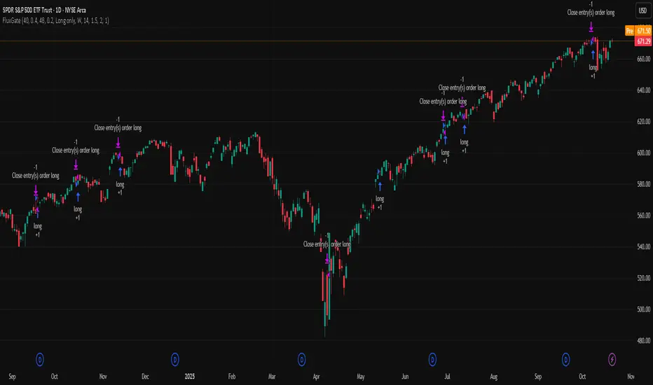
FluxGate Daily Swing StrategySummary in one paragraph
FluxGate treats long and short as different ecosystems. It runs two independent engines so the long side can be bold when the tape rewards upside persistence while the short side can stay selective when downside is messy. The core reads three directional drivers from price geometry then removes overlap before gating with clean path checks. The complementary risk module anchors stop distance to a higher timeframe ATR so a unit means the same thing on SPY and BTC. It can add take profit breakeven and an ATR trail that only activates after the trade earns it. If a stop is hit the strategy can re enter in the same direction on the next bar with a daily retry cap that you control. Add it to a clean chart. Use defaults to see the intended behavior. For conservative workflows evaluate on bar close.
Scope and intent
• Markets. Large cap equities and liquid ETFs major FX pairs US index futures and liquid crypto pairs
• Timeframes. From one minute to daily
• Default demo in this publication. SPY on one day timeframe
• Purpose. Reduce false starts without missing sustained trends by fusing independent drivers and suppressing activity when the path is noisy
• Limits. This is a strategy. Orders are simulated on standard candles. Non standard chart types are not supported for execution
Originality and usefulness
• Unique fusion. FluxGate extracts three drivers that look at price from different angles. Direction measures slope of a smoothed guide and scales by realized volatility so a point of slope does not mean a different thing on different symbols. Persistence looks at short sign agreement to reward series of closes that keep direction. Curvature measures the second difference of a local fit to wake up during convex pushes. These three are then orthonormalized so a strong reading in one does not double count through another.
• Gates that matter. Efficiency ratio prefers direct paths over treadmills. Entropy turns up versus down frequency into an information read. Light fractal cohesion punishes wrinkly paths. Together they slow the system in chop and allow it to open up when the path is clean.
• Separate long and short engines. Threshold tilts adapt to the skew of score excursions. That lets long engage earlier when upside distribution supports it and keeps short cautious where downside surprise and venue frictions are common.
• Practical risk behavior. Stops are ATR anchored on a higher timeframe so the unit is portable. Take profit is expressed in R so two R means the same concept across symbols. Breakeven and trailing only activate after a chosen R so early noise does not squeeze a good entry. Re entry after stop lets the system try again without you babysitting the chart.
• Testability. Every major window and the aggression controls live in Inputs. There is no hidden magic number.
Method overview in plain language
Base measures
• Return basis. Natural log of close over prior close for stability and easy aggregation through time. Realized volatility is the standard deviation of returns over a moving window.
• Range basis for risk. ATR computed on a higher timeframe anchor such as day week or month. That anchor is steady across venues and avoids chasing chart specific quirks.
Components
• Directional intensity. Use an EMA of typical price as a guide. Take the day to day slope as raw direction. Divide by realized volatility to get a unit free measure. Soft clip to keep outliers from dominating.
• Persistence. Encode whether each bar closed up or down. Measure short sign agreement so a string of higher closes scores better than a jittery sequence. This favors push continuity without guessing tops or bottoms.
• Curvature. Fit a short linear regression and compute the second difference of the fitted series. Strong curvature flags acceleration that slope alone may miss.
• Efficiency gate. Compare net move to path length over a gate window. Values near one indicate direct paths. Values near zero indicate treadmill behavior.
• Entropy gate. Convert up versus down frequency into a probability of direction. High entropy means coin toss. The gate narrows there.
• Fractal cohesion. A light read of path wrinkliness relative to span. Lower cohesion reduces the urge to act.
• Phase assist. Map price inside a recent channel to a small signed bias that grows with confidence. This helps entries lean toward the right half of the channel without becoming a breakout rule.
• Shock control. Compare short volatility to long volatility. When short term volatility spikes the shock gate temporarily damps activity so the system waits for pressure to normalize.
Fusion rule
• Normalize the three drivers after removing overlap
• Blend with weights that adapt to your aggression input
• Multiply by the gates to respect path quality
• Smooth just enough to avoid jitter while keeping timing responsive
• Compute an adaptive mean and deviation of the score and set separate long and short thresholds with a small tilt informed by skew sign
• The result is one long score and one short score that can cross their thresholds at different times for the same tape which is a feature not a bug
Signal rule
• A long suggestion appears when the long score crosses above its long threshold while all gates are active
• A short suggestion appears when the short score crosses below its short threshold while all gates are active
• If any required gate is missing the state is wait
• When a position is open the status is in long or in short until the complementary risk engine exits or your entry mode closes and flips
Inputs with guidance
Setup Long
• Base length Long. Master window for the long engine. Typical range twenty four to eighty. Raising it improves selectivity and reduces trade count. Lowering it reacts faster but can increase noise
• Aggression Long. Zero to one. Higher values make thresholds more permissive and shorten smoothing
Setup Short
• Base length Short. Master window for the short engine. Typical range twenty eight to ninety six
• Aggression Short. Zero to one. Lower values keep shorts conservative which is often useful on upward drifting symbols
Entries and UI
• Entry mode. Both or Long only or Short only
Complementary risk engine
• Enable risk engine. Turns on bracket exits while keeping your signal logic untouched
• ATR anchor timeframe. Day Week or Month. This sets the structural unit of stop distance
• ATR length. Default fourteen
• Stop multiple. Default one point five times the anchor ATR
• Use take profit. On by default
• Take profit in R. Default two R
• Breakeven trigger in R. Default one R
Usage recipes
Intraday trend focus
• Entry mode Both
• ATR anchor Week
• Aggression Long zero point five Aggression Short zero point three
• Stop multiple one point five Take profit two R
• Expect fewer trades that stick to directional pushes and skip treadmill noise
Intraday mean reversion focus
• Session windows optional if you add them in your copy
• ATR anchor Day
• Lower aggression both sides
• Breakeven later and trailing later so the first bounce has room
• This favors fade entries that still convert into trends when the path stays clean
Swing continuation
• Signal timeframe four hours or one day
• Confirm timeframe one day if you choose to include bias
• ATR anchor Week or Month
• Larger base windows and a steady two R target
• This accepts fewer entries and aims for larger holds
Properties visible in this publication
• Initial capital 25.000
• Base currency USD
• Default order size percent of equity value three - 3% of the total capital
• Pyramiding zero
• Commission zero point zero three percent - 0.03% of total capital
• Slippage five ticks
• Process orders on close off
• Recalculate after order is filled off
• Calc on every tick off
• Bar magnifier off
• Any request security calls use lookahead off everywhere
Realism and responsible publication
• No performance promises. Past results never guarantee future outcomes
• Fills and slippage vary by venue and feed
• Strategies run on standard candles only
• Shapes can update while a bar is forming and settle on close
• Keep risk per trade sensible. Around one percent is typical for study. Above five to ten percent is rarely sustainable
Honest limitations and failure modes
• Sudden news and thin liquidity can break assumptions behind entropy and cohesion reads
• Gap heavy symbols often behave better with a True Range basis for risk than a simple range
• Very quiet regimes can reduce score contrast. Consider longer windows or higher thresholds when markets sleep
• Session windows follow the exchange time of the chart if you add them
• If stop and target can both be inside a single bar this strategy prefers stop first to keep accounting conservative
Open source reuse and credits
• No reused open source beyond public domain building blocks such as ATR EMA and linear regression concepts
Legal
Education and research only. Not investment advice. You are responsible for your decisions. Test on history and in simulation with realistic costs
Quantum Flux Universal Strategy Summary in one paragraph
Quantum Flux Universal is a regime switching strategy for stocks, ETFs, index futures, major FX pairs, and liquid crypto on intraday and swing timeframes. It helps you act only when the normalized core signal and its guide agree on direction. It is original because the engine fuses three adaptive drivers into the smoothing gains itself. Directional intensity is measured with binary entropy, path efficiency shapes trend quality, and a volatility squash preserves contrast. Add it to a clean chart, watch the polarity lane and background, and trade from positive or negative alignment. For conservative workflows use on bar close in the alert settings when you add alerts in a later version.
Scope and intent
• Markets. Large cap equities and ETFs. Index futures. Major FX pairs. Liquid crypto
• Timeframes. One minute to daily
• Default demo used in the publication. QQQ on one hour
• Purpose. Provide a robust and portable way to detect when momentum and confirmation align, while dampening chop and preserving turns
• Limits. This is a strategy. Orders are simulated on standard candles only
Originality and usefulness
• Unique concept or fusion. The novelty sits in the gain map. Instead of gating separate indicators, the model mixes three drivers into the adaptive gains that power two one pole filters. Directional entropy measures how one sided recent movement has been. Kaufman style path efficiency scores how direct the path has been. A volatility squash stabilizes step size. The drivers are blended into the gains with visible inputs for strength, windows, and clamps.
• What failure mode it addresses. False starts in chop and whipsaw after fast spikes. Efficiency and the squash reduce over reaction in noise.
• Testability. Every component has an input. You can lengthen or shorten each window and change the normalization mode. The polarity plot and background provide a direct readout of state.
• Portable yardstick. The core is normalized with three options. Z score, percent rank mapped to a symmetric range, and MAD based Z score. Clamp bounds define the effective unit so context transfers across symbols.
Method overview in plain language
The strategy computes two smoothed tracks from the chart price source. The fast track and the slow track use gains that are not fixed. Each gain is modulated by three drivers. A driver for directional intensity, a driver for path efficiency, and a driver for volatility. The difference between the fast and the slow tracks forms the raw flux. A small phase assist reduces lag by subtracting a portion of the delayed value. The flux is then normalized. A guide line is an EMA of a small lead on the flux. When the flux and its guide are both above zero, the polarity is positive. When both are below zero, the polarity is negative. Polarity changes create the trade direction.
Base measures
• Return basis. The step is the change in the chosen price source. Its absolute value feeds the volatility estimate. Mean absolute step over the window gives a stable scale.
• Efficiency basis. The ratio of net move to the sum of absolute step over the window gives a value between zero and one. High values mean trend quality. Low values mean chop.
• Intensity basis. The fraction of up moves over the window plugs into binary entropy. Intensity is one minus entropy, which maps to zero in uncertainty and one in very one sided moves.
Components
• Directional Intensity. Measures how one sided recent bars have been. Smoothed with RMA. More intensity increases the gain and makes the fast and slow tracks react sooner.
• Path Efficiency. Measures the straightness of the price path. A gamma input shapes the curve so you can make trend quality count more or less. Higher efficiency lifts the gain in clean trends.
• Volatility Squash. Normalizes the absolute step with Z score then pushes it through an arctangent squash. This caps the effect of spikes so they do not dominate the response.
• Normalizer. Three modes. Z score for familiar units, percent rank for a robust monotone map to a symmetric range, and MAD based Z for outlier resistance.
• Guide Line. EMA of the flux with a small lead term that counteracts lag without heavy overshoot.
Fusion rule
• Weighted sum of the three drivers with fixed weights visible in the code comments. Intensity has fifty percent weight. Efficiency thirty percent. Volatility twenty percent.
• The blend power input scales the driver mix. Zero means fixed spans. One means full driver control.
• Minimum and maximum gain clamps bound the adaptive gain. This protects stability in quiet or violent regimes.
Signal rule
• Long suggestion appears when flux and guide are both above zero. That sets polarity to plus one.
• Short suggestion appears when flux and guide are both below zero. That sets polarity to minus one.
• When polarity flips from plus to minus, the strategy closes any long and enters a short.
• When flux crosses above the guide, the strategy closes any short.
What you will see on the chart
• White polarity plot around the zero line
• A dotted reference line at zero named Zen
• Green background tint for positive polarity and red background tint for negative polarity
• Strategy long and short markers placed by the TradingView engine at entry and at close conditions
• No table in this version to keep the visual clean and portable
Inputs with guidance
Setup
• Price source. Default ohlc4. Stable for noisy symbols.
• Fast span. Typical range 6 to 24. Raising it slows the fast track and can reduce churn. Lowering it makes entries more reactive.
• Slow span. Typical range 20 to 60. Raising it lengthens the baseline horizon. Lowering it brings the slow track closer to price.
Logic
• Guide span. Typical range 4 to 12. A small guide smooths without eating turns.
• Blend power. Typical range 0.25 to 0.85. Raising it lets the drivers modulate gains more. Lowering it pushes behavior toward fixed EMA style smoothing.
• Vol window. Typical range 20 to 80. Larger values calm the volatility driver. Smaller values adapt faster in intraday work.
• Efficiency window. Typical range 10 to 60. Larger values focus on smoother trends. Smaller values react faster but accept more noise.
• Efficiency gamma. Typical range 0.8 to 2.0. Above one increases contrast between clean trends and chop. Below one flattens the curve.
• Min alpha multiplier. Typical range 0.30 to 0.80. Lower values increase smoothing when the mix is weak.
• Max alpha multiplier. Typical range 1.2 to 3.0. Higher values shorten smoothing when the mix is strong.
• Normalization window. Typical range 100 to 300. Larger values reduce drift in the baseline.
• Normalization mode. Z score, percent rank, or MAD Z. Use MAD Z for outlier heavy symbols.
• Clamp level. Typical range 2.0 to 4.0. Lower clamps reduce the influence of extreme runs.
Filters
• Efficiency filter is implicit in the gain map. Raising efficiency gamma and the efficiency window increases the preference for clean trends.
• Micro versus macro relation is handled by the fast and slow spans. Increase separation for swing, reduce for scalping.
• Location filter is not included in v1.0. If you need distance gates from a reference such as VWAP or a moving mean, add them before publication of a new version.
Alerts
• This version does not include alertcondition lines to keep the core minimal. If you prefer alerts, add names Long Polarity Up, Short Polarity Down, Exit Short on Flux Cross Up in a later version and select on bar close for conservative workflows.
Strategy has been currently adapted for the QQQ asset with 30/60min timeframe.
For other assets may require new optimization
Properties visible in this publication
• Initial capital 25000
• Base currency Default
• Default order size method percent of equity with value 5
• Pyramiding 1
• Commission 0.05 percent
• Slippage 10 ticks
• Process orders on close ON
• Bar magnifier ON
• Recalculate after order is filled OFF
• Calc on every tick OFF
Honest limitations and failure modes
• Past results do not guarantee future outcomes
• Economic releases, circuit breakers, and thin books can break the assumptions behind intensity and efficiency
• Gap heavy symbols may benefit from the MAD Z normalization
• Very quiet regimes can reduce signal contrast. Use longer windows or higher guide span to stabilize context
• Session time is the exchange time of the chart
• If both stop and target can be hit in one bar, tie handling would matter. This strategy has no fixed stops or targets. It uses polarity flips for exits. If you add stops later, declare the preference
Open source reuse and credits
• None beyond public domain building blocks and Pine built ins such as EMA, SMA, standard deviation, RMA, and percent rank
• Method and fusion are original in construction and disclosure
Legal
Education and research only. Not investment advice. You are responsible for your decisions. Test on historical data and in simulation before any live use. Use realistic costs.
Strategy add on block
Strategy notice
Orders are simulated by the TradingView engine on standard candles. No request.security() calls are used.
Entries and exits
• Entry logic. Enter long when both the normalized flux and its guide line are above zero. Enter short when both are below zero
• Exit logic. When polarity flips from plus to minus, close any long and open a short. When the flux crosses above the guide line, close any short
• Risk model. No initial stop or target in v1.0. The model is a regime flipper. You can add a stop or trail in later versions if needed
• Tie handling. Not applicable in this version because there are no fixed stops or targets
Position sizing
• Percent of equity in the Properties panel. Five percent is the default for examples. Risk per trade should not exceed five to ten percent of equity. One to two percent is a common choice
Properties used on the published chart
• Initial capital 25000
• Base currency Default
• Default order size percent of equity with value 5
• Pyramiding 1
• Commission 0.05 percent
• Slippage 10 ticks
• Process orders on close ON
• Bar magnifier ON
• Recalculate after order is filled OFF
• Calc on every tick OFF
Dataset and sample size
• Test window Jan 2, 2014 to Oct 16, 2025 on QQQ one hour
• Trade count in sample 324 on the example chart
Release notes template for future updates
Version 1.1.
• Add alertcondition lines for long, short, and exit short
• Add optional table with component readouts
• Add optional stop model with a distance unit expressed as ATR or a percent of price
Notes. Backward compatibility Yes. Inputs migrated Yes.

Apex Edge – Wolfe Wave HunterApex Edge – Wolfe Wave Hunter
The modern Wolfe Wave, rebuilt for the algo era
This isn’t just another Wolfe Wave indicator. Classic Wolfe detection is rigid, outdated, and rarely tradable. Apex Edge – Wolfe Wave Hunter re-engineers the pattern into a modern, SMC-driven model that adapts to today’s liquidity-dominated markets. It’s not about drawing pretty shapes – it’s about extracting precision entries with asymmetric risk-to-reward potential.
🔎 What it does
Automatic Wolfe Wave Detection
Identifies bullish and bearish Wolfe Wave structures using pivot-based logic, symmetry filters, and slope tolerances.
Channel Glow Zones
Highlights the Wolfe channel and projects it forward into the future (bars are user-defined). This allows you to see the full potential of the trade before price even begins its move.
Stop Loss (SL) & Entry Arrow
At the completion of Wave 5, the algo prints a Stop Loss line and a tiny entry arrow (green for bullish, red for bearish). but the colours can be changed in user settings. This is the “execution point” — where the Wolfe setup becomes tradable.
Target Projection Lines
TP1 (EPA): Derived from the traditional 1–4 line projection.
TP2 (1.272 Fib): Optional secondary profit target.
TP3 (1.618 Fib): Optional extended target for large runners.
All TP lines extend into the future, so you can track them as price evolves.
Volume Confirmation (optional)
A relative volume filter ensures Wave 5 is formed with meaningful market participation before a setup is confirmed.
Alerts (ready out of the box)
Custom alerts can be fired whenever a bullish or bearish Wolfe Wave is confirmed. No need to babysit the charts — let the script notify you.
⚙️ Customisation & User Control
Every trader’s market and style is different. That’s why Wolfe Wave Hunter is fully customisable:
Arrow Colours & Size
Works on both light and dark charts. Choose your own bullish/bearish entry arrow colours for maximum visibility.
Tolerance Levels
Adjust symmetry and slope tolerance to refine how strict the channel rules are.
Tighter settings = fewer but cleaner zones.
Looser settings = more frequent setups, but with slightly lower structural quality.
Channel Glow Projection
Define how many bars forward the channel is drawn. This controls how far into the future your Wolfe zones are extended.
Stop Loss Line Length
Keep the SL visible without it extending infinitely across your chart.
Take Profit Line Colors
Each TP projection can be styled to your preference, allowing you to clearly separate TP1, TP2, and TP3.
This isn’t a one-size-fits-all tool. You can shape Wolfe detection logic to match the pairs, timeframes, and market conditions you trade most.
🚀 Why it’s different
Classic Wolfe waves are rare — this script adapts the model into something practical and tradeable in modern markets.
Liquidity-aligned — many setups align with structural sweeps of Wave 3 liquidity before driving into profit.
Entry built-in — most Wolfe scripts only draw the structure. Wolfe Wave Hunter gives you a precise entry point, SL, and projected TPs.
Backtest-friendly — you’ll quickly discover which assets respect Wolfe waves and which don’t, creating your own high-probability Wolfe watchlist.
⚠️ Limitations & Disclaimer
Not all markets respect Wolfe Waves. Some FX pairs, metals, and indices respect the structure beautifully; others do not. Backtest and create your own shortlist.
No guaranteed sweeps. Many entries occur after a liquidity sweep of Wave 3, but not all. The algo is designed to detect Wolfe completion, not enforce textbook liquidity rules.
Probabilistic, not predictive. Wolfe setups don’t win every time. Always use risk management.
High-RR focus. This is not a high-frequency tool. It’s designed for precision, asymmetric setups where risk is small and reward potential is large.
✅ The Bottom Line
Apex Edge – Wolfe Wave Hunter is a modern reimagination of the Wolfe Wave. It blends structural geometry, liquidity dynamics, and algo-driven execution into a single tool that:
Detects the pattern automatically
Provides SL, entry, and TP levels
Offers alerts for hands-off trading
Allows deep customisation for different markets
When it hits, it delivers outstanding risk-to-reward. Backtest, refine your tolerances, and build your watchlist of assets where Wolfe structures consistently pay.
This isn’t just Wolfe detection — it’s Wolfe trading, rebuilt for the modern trader.
Developer Notes - As always with the Apex Edge Brand, user feedback and recommendations will always be respected. Simply drop us a message with your comments and we will endeavour to address your needs in future version updates.
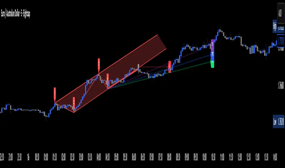
Extremum Range MA Crossover Strategy1. Principle of Work & Strategy Logic ⚙️📈
Main idea: The strategy tries to catch the moment of a breakout from a price consolidation range (flat) and the start of a new trend. It combines two key elements:
Moving Average (MA) 📉: Acts as a dynamic support/resistance level and trend filter.
Range Extremes (Range High/Low) 🔺🔻: Define the borders of the recent price channel or consolidation.
The strategy does not attempt to catch absolute tops and bottoms. Instead, it enters an already formed move after the breakout, expecting continuation.
Type: Trend-following, momentum-based.
Timeframes: Works on different TFs (H1, H4, D), but best suited for H4 and higher, where breakouts are more meaningful.
2. Justification of Indicators & Settings ⚙️
A. Moving Average (MA) 📊
Why used: Core of the strategy. It smooths price fluctuations and helps define the trend. The price (via extremes) must cross the MA → signals a potential trend shift or strengthening.
Parameters:
maLength = 20: Default length (≈ one trading month, 20-21 days). Good balance between sensitivity & smoothing.
Lower TF → reduce (10–14).
Higher TF → increase (50).
maSource: Defines price source (default = Close). Alternatives (HL2, HLC3) → smoother, less noisy MA.
maType: Default = EMA (Exponential MA).
Why EMA? Faster reaction to recent price changes vs SMA → useful for breakout strategies.
Other options:
SMA 🟦 – classic, slowest.
WMA 🟨 – weights recent data stronger.
HMA 🟩 – near-zero lag, but “nervous,” more false signals.
DEMA/TEMA 🟧 – even faster & more sensitive than EMA.
VWMA 🔊 – volume-weighted.
ZLEMA ⏱ – reduced lag.
👉 Choice = tradeoff between speed of reaction & false signals.
B. Range Extremes (Previous High/Low) 📏
Why used: Define borders of recent trading range.
prevHigh = local resistance.
prevLow = local support.
Break of these levels on close = trigger.
Parameters:
lookbackPeriod = 5: Searches for highest high / lowest low of last 5 candles. Very recent range.
Higher value (10–20) → wider, stronger ranges but rarer signals.
3. Entry & Exit Rules 🎯
Long signals (BUY) 🟢📈
Condition (longCondition): Previous Low crosses MA from below upwards.
→ Price bounced from the bottom & strong enough to push range border above MA.
Execution: Auto-close short (if any) → open long.
Short signals (SELL) 🔴📉
Condition (shortCondition): Previous High crosses MA from above downwards.
→ Price rejected from the top, upper border failed above MA.
Execution: Auto-close long (if any) → open short.
Exit conditions 🚪
Exit Long (exitLongCondition): Close below prevLow.
→ Uptrend likely ended, range shifts down.
Exit Short (exitShortCondition): Close above prevHigh.
→ Downtrend likely ended, range shifts up.
⚠️ Important: Exit = only on candle close beyond extremes (not just wick).
4. Trading Settings ⚒️
overlay = true → indicators shown on chart.
initial_capital = 10000 💵.
default_qty_type = strategy.cash, default_qty_value = 100 → trades fixed $100 per order (not lots). Can switch to % of equity.
commission_type = strategy.commission.percent, commission_value = 0.1 → default broker fee = 0.1%. Adjust for your broker!
slippage = 3 → slippage = 3 ticks. Adjust to asset liquidity.
currency = USD.
margin_long = 100, margin_short = 100 → no leverage (100% margin).
5. Visualization on Chart 📊
The strategy draws 3 lines:
🔵 MA line (thickness 2).
🔴 Previous High (last N candles).
🟢 Previous Low (last N candles).
Also: entry/exit arrows & equity curve shown in backtest.
Disclaimer ⚠️📌
Risk Warning: This description & code are for educational purposes only. Not financial advice. Trading (Forex, Stocks, Crypto) carries high risk and may lead to full capital loss. You trade at your own risk.
Testing: Always backtest & demo test first. Past results ≠ future profits.
Responsibility: Author of this strategy & description is not responsible for your trading decisions or losses.

BE-Fib Channel 2 Sided Trading█ Overview:
"BE-Fib Channel 2 Sided Trading" indicator is built with the thought of 2 profound setups named "Cup & Handle (C&H)" and "Fibonacci Channel Trading (FCT)" with the context of "day trading" or with a minimum holding period.
█ Similarities, Day Trading Context & Error Patterns:
While the known fact is that both C&H and FCT provide setups with lesser risk with bigger returns, they both share the similar "Base Pattern".
Note: Inverse of the above Image shall switch the setups between long vs short.
Since the indicator is designed for smaller time-frame candles, there may be instances where the "base pattern" does not visually resemble a Cup & Handle (C&H) pattern. However, patterns are validated using pivot points. The points labeled "A" and "C" can be equal or slightly slanted. Settings of the Indicator allows traders a flexibility to control the angle of these points to spot the strategies according to set conditions. Therefore, understanding the nuances of these patterns is crucial for effective decision-making.
█ 2 Sided Edge: FCT suggests to take trade closer to the yellow line to get better RR ratio. this leaves a small chance of doubt as to; what if price is intended to break the Yellow line thereby activating the C&H.
Wait for the confirmation is a Big FOMO with a compromised RR.
Hence, This indicator is designed to handle both the patterns based on the strength, FIFO and pattern occurring delay.
█ How to Use this Indicator:
Step 1: Enable the Show Sample Sensitivity option to understand the angle of yellow line shown in the sample image. By enabling this option, On the last bar you shall see 4 lines being plotted depicting the max angle which is acceptable for both long and short trades.
Note: Angle can be controlled via setting "Sensitivity".
Higher Sensitivity --> Higher Setup identification --> can lead to failed setups due to 2 sided trading.
Lower Sensitivity --> Lower Setup identification --> can increase the changes of being right.
Step 2: Adjust the look back & look forward periods which shall be used for identifying patterns.
Note: Smaller values can lead to more setups being identified but can hamper the performance of the indicator while increasing the chances of failures. larger values identifies more significant setup but leads to more waiting period thereby compromising on the RR.
Step 3: Adjust the Base Range.
Note: Smaller values can lead to more setups being identified but can hamper the performance of the indicator while increasing the chances of failures. larger values identifies more significant setup but leads to more Risk on play.
Step 4: set the Entry level for FCT & Set the SL for Both FCT & C&H and Target Reward ratio for C&H.
█ Features of Indicator & How it works:
1. Patterns are being identified using Pivot Points method.
2. Tracks & validates both the setups simultaneously on every candle and traded one at a time based on FIFO, New setups found in-between, Defined Entry Levels while on wait for the other pattern to get activated.
3. Alerts added for trade events.
4. FCT setups are generally traded with trailed SL level and increasing Target level on every completed bar. while C&H has the standard SL & TP level with no Trail SL option.
DISCLAIMER: No sharing, copying, reselling, modifying, or any other forms of use are authorized for our documents, script / strategy, and the information published with them. This informational planning script / strategy is strictly for individual use and educational purposes only. This is not financial or investment advice. Investments are always made at your own risk and are based on your personal judgement. I am not responsible for any losses you may incur. Please invest wisely.
Happy to receive suggestions and feedback in order to improve the performance of the indicator better.
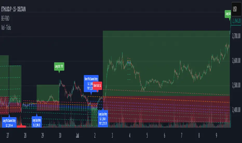
PnL Bubble [%] | Fractalyst1. What's the indicator purpose?
The PnL Bubble indicator transforms your strategy's trade PnL percentages into an interactive bubble chart with professional-grade statistics and performance analytics. It helps traders quickly assess system profitability, understand win/loss distribution patterns, identify outliers, and make data-driven strategy improvements.
How does it work?
Think of this indicator as a visual report card for your trading performance. Here's what it does:
What You See
Colorful Bubbles: Each bubble represents one of your trades
Blue/Cyan bubbles = Winning trades (you made money)
Red bubbles = Losing trades (you lost money)
Bigger bubbles = Bigger wins or losses
Smaller bubbles = Smaller wins or losses
How It Organizes Your Trades:
Like a Photo Album: Instead of showing all your trades at once (which would be messy), it shows them in "pages" of 500 trades each:
Page 1: Your first 500 trades
Page 2: Trades 501-1000
Page 3: Trades 1001-1500, etc.
What the Numbers Tell You:
Average Win: How much money you typically make on winning trades
Average Loss: How much money you typically lose on losing trades
Expected Value (EV): Whether your trading system makes money over time
Positive EV = Your system is profitable long-term
Negative EV = Your system loses money long-term
Payoff Ratio (R): How your average win compares to your average loss
R > 1 = Your wins are bigger than your losses
R < 1 = Your losses are bigger than your wins
Why This Matters:
At a Glance: You can instantly see if you're a profitable trader or not
Pattern Recognition: Spot if you have more big wins than big losses
Performance Tracking: Watch how your trading improves over time
Realistic Expectations: Understand what "average" performance looks like for your system
The Cool Visual Effects:
Animation: The bubbles glow and shimmer to make the chart more engaging
Highlighting: Your biggest wins and losses get extra attention with special effects
Tooltips: hover any bubble to see details about that specific trade.
What are the underlying calculations?
The indicator processes trade PnL data using a dual-matrix architecture for optimal performance:
Dual-Matrix System:
• Display Matrix (display_matrix): Bounded to 500 trades for rendering performance
• Statistics Matrix (stats_matrix): Unbounded storage for complete statistical accuracy
Trade Classification & Aggregation:
// Separate wins, losses, and break-even trades
if val > 0.0
pos_sum += val // Sum winning trades
pos_count += 1 // Count winning trades
else if val < 0.0
neg_sum += val // Sum losing trades
neg_count += 1 // Count losing trades
else
zero_count += 1 // Count break-even trades
Statistical Averages:
avg_win = pos_count > 0 ? pos_sum / pos_count : na
avg_loss = neg_count > 0 ? math.abs(neg_sum) / neg_count : na
Win/Loss Rates:
total_obs = pos_count + neg_count + zero_count
win_rate = pos_count / total_obs
loss_rate = neg_count / total_obs
Expected Value (EV):
ev_value = (avg_win × win_rate) - (avg_loss × loss_rate)
Payoff Ratio (R):
R = avg_win ÷ |avg_loss|
Contribution Analysis:
ev_pos_contrib = avg_win × win_rate // Positive EV contribution
ev_neg_contrib = avg_loss × loss_rate // Negative EV contribution
How to integrate with any trading strategy?
Equity Change Tracking Method:
//@version=6
strategy("Your Strategy with Equity Change Export", overlay=true)
float prev_trade_equity = na
float equity_change_pct = na
if barstate.isconfirmed and na(prev_trade_equity)
prev_trade_equity := strategy.equity
trade_just_closed = strategy.closedtrades != strategy.closedtrades
if trade_just_closed and not na(prev_trade_equity)
current_equity = strategy.equity
equity_change_pct := ((current_equity - prev_trade_equity) / prev_trade_equity) * 100
prev_trade_equity := current_equity
else
equity_change_pct := na
plot(equity_change_pct, "Equity Change %", display=display.data_window)
Integration Steps:
1. Add equity tracking code to your strategy
2. Load both strategy and PnL Bubble indicator on the same chart
3. In bubble indicator settings, select your strategy's equity tracking output as data source
4. Configure visualization preferences (colors, effects, page navigation)
How does the pagination system work?
The indicator uses an intelligent pagination system to handle large trade datasets efficiently:
Page Organization:
• Page 1: Trades 1-500 (most recent)
• Page 2: Trades 501-1000
• Page 3: Trades 1001-1500
• Page N: Trades to
Example: With 1,500 trades total (3 pages available):
• User selects Page 1: Shows trades 1-500
• User selects Page 4: Automatically falls back to Page 3 (trades 1001-1500)
5. Understanding the Visual Elements
Bubble Visualization:
• Color Coding: Cyan/blue gradients for wins, red gradients for losses
• Size Mapping: Bubble size proportional to trade magnitude (larger = bigger P&L)
• Priority Rendering: Largest trades displayed first to ensure visibility
• Gradient Effects: Color intensity increases with trade magnitude within each category
Interactive Tooltips:
Each bubble displays quantitative trade information:
tooltip_text = outcome + " | PnL: " + pnl_str +
" Date: " + date_str + " " + time_str +
" Trade #" + str.tostring(trade_number) + " (Page " + str.tostring(active_page) + ")" +
" Rank: " + str.tostring(rank) + " of " + str.tostring(n_display_rows) +
" Percentile: " + str.tostring(percentile, "#.#") + "%" +
" Magnitude: " + str.tostring(magnitude_pct, "#.#") + "%"
Example Tooltip:
Win | PnL: +2.45%
Date: 2024.03.15 14:30
Trade #1,247 (Page 3)
Rank: 5 of 347
Percentile: 98.6%
Magnitude: 85.2%
Reference Lines & Statistics:
• Average Win Line: Horizontal reference showing typical winning trade size
• Average Loss Line: Horizontal reference showing typical losing trade size
• Zero Line: Threshold separating wins from losses
• Statistical Labels: EV, R-Ratio, and contribution analysis displayed on chart
What do the statistical metrics mean?
Expected Value (EV):
Represents the mathematical expectation per trade in percentage terms
EV = (Average Win × Win Rate) - (Average Loss × Loss Rate)
Interpretation:
• EV > 0: Profitable system with positive mathematical expectation
• EV = 0: Break-even system, profitability depends on execution
• EV < 0: Unprofitable system with negative mathematical expectation
Example: EV = +0.34% means you expect +0.34% profit per trade on average
Payoff Ratio (R):
Quantifies the risk-reward relationship of your trading system
R = Average Win ÷ |Average Loss|
Interpretation:
• R > 1.0: Wins are larger than losses on average (favorable risk-reward)
• R = 1.0: Wins and losses are equal in magnitude
• R < 1.0: Losses are larger than wins on average (unfavorable risk-reward)
Example: R = 1.5 means your average win is 50% larger than your average loss
Contribution Analysis (Σ):
Breaks down the components of expected value
Positive Contribution (Σ+) = Average Win × Win Rate
Negative Contribution (Σ-) = Average Loss × Loss Rate
Purpose:
• Shows how much wins contribute to overall expectancy
• Shows how much losses detract from overall expectancy
• Net EV = Σ+ - Σ- (Expected Value per trade)
Example: Σ+: 1.23% means wins contribute +1.23% to expectancy
Example: Σ-: -0.89% means losses drag expectancy by -0.89%
Win/Loss Rates:
Win Rate = Count(Wins) ÷ Total Trades
Loss Rate = Count(Losses) ÷ Total Trades
Shows the probability of winning vs losing trades
Higher win rates don't guarantee profitability if average losses exceed average wins
7. Demo Mode & Synthetic Data Generation
When using built-in sources (close, open, etc.), the indicator generates realistic demo trades for testing:
if isBuiltInSource(source_data)
// Generate random trade outcomes with realistic distribution
u_sign = prand(float(time), float(bar_index))
if u_sign < 0.5
v_push := -1.0 // Loss trade
else
// Skewed distribution favoring smaller wins (realistic)
u_mag = prand(float(time) + 9876.543, float(bar_index) + 321.0)
k = 8.0 // Skewness factor
t = math.pow(u_mag, k)
v_push := 2.5 + t * 8.0 // Win trade
Demo Characteristics:
• Realistic win/loss distribution mimicking actual trading patterns
• Skewed distribution favoring smaller wins over large wins
• Deterministic randomness for consistent demo results
• Includes jitter effects to prevent visual overlap
8. Performance Limitations & Optimizations
Display Constraints:
points_count = 500 // Maximum 500 dots per page for optimal performance
Pine Script v6 Limits:
• Label Count: Maximum 500 labels per indicator
• Line Count: Maximum 100 lines per indicator
• Box Count: Maximum 50 boxes per indicator
• Matrix Size: Efficient memory management with dual-matrix system
Optimization Strategies:
• Pagination System: Handle unlimited trades through 500-trade pages
• Priority Rendering: Largest trades displayed first for maximum visibility
• Dual-Matrix Architecture: Separate display (bounded) from statistics (unbounded)
• Smart Fallback: Automatic page clamping prevents empty displays
Impact & Workarounds:
• Visual Limitation: Only 500 trades visible per page
• Statistical Accuracy: Complete dataset used for all calculations
• Navigation: Use page input to browse through entire trade history
• Performance: Smooth operation even with thousands of trades
9. Statistical Accuracy Guarantees
Data Integrity:
• Complete Dataset: Statistics matrix stores ALL trades without limit
• Proper Aggregation: Separate tracking of wins, losses, and break-even trades
• Mathematical Precision: Pine Script v6's enhanced floating-point calculations
• Dual-Matrix System: Display limitations don't affect statistical accuracy
Calculation Validation:
// Verified formulas match standard trading mathematics
avg_win = pos_sum / pos_count // Standard average calculation
win_rate = pos_count / total_obs // Standard probability calculation
ev_value = (avg_win * win_rate) - (avg_loss * loss_rate) // Standard EV formula
Accuracy Features:
• Mathematical Correctness: Formulas follow established trading statistics
• Data Preservation: Complete dataset maintained for all calculations
• Precision Handling: Proper rounding and boundary condition management
• Real-Time Updates: Statistics recalculated on every new trade
10. Advanced Technical Features
Real-Time Animation Engine:
// Shimmer effects with sine wave modulation
offset = math.sin(shimmer_t + phase) * amp
// Dynamic transparency with organic flicker
new_transp = math.min(flicker_limit, math.max(-flicker_limit, cur_transp + dir * flicker_step))
• Sine Wave Shimmer: Dynamic glowing effects on bubbles
• Organic Flicker: Random transparency variations for natural feel
• Extreme Value Highlighting: Special visual treatment for outliers
• Smooth Animations: Tick-based updates for fluid motion
Magnitude-Based Priority Rendering:
// Sort trades by magnitude for optimal visual hierarchy
sort_indices_by_magnitude(values_mat)
• Largest First: Most important trades always visible
• Intelligent Sorting: Custom bubble sort algorithm for trade prioritization
• Performance Optimized: Efficient sorting for real-time updates
• Visual Hierarchy: Ensures critical trades never get hidden
Professional Tooltip System:
• Quantitative Data: Pure numerical information without interpretative language
• Contextual Ranking: Shows trade position within page dataset
• Percentile Analysis: Performance ranking as percentage
• Magnitude Scaling: Relative size compared to page maximum
• Professional Format: Clean, data-focused presentation
11. Quick Start Guide
Step 1: Add Indicator
• Search for "PnL Bubble | Fractalyst" in TradingView indicators
• Add to your chart (works on any timeframe)
Step 2: Configure Data Source
• Demo Mode: Leave source as "close" to see synthetic trading data
• Strategy Mode: Select your strategy's PnL% output as data source
Step 3: Customize Visualization
• Colors: Set positive (cyan), negative (red), and neutral colors
• Page Navigation: Use "Trade Page" input to browse trade history
• Visual Effects: Built-in shimmer and animation effects are enabled by default
Step 4: Analyze Performance
• Study bubble patterns for win/loss distribution
• Review statistical metrics: EV, R-Ratio, Win Rate
• Use tooltips for detailed trade analysis
• Navigate pages to explore full trade history
Step 5: Optimize Strategy
• Identify outlier trades (largest bubbles)
• Analyze risk-reward profile through R-Ratio
• Monitor Expected Value for system profitability
• Use contribution analysis to understand win/loss impact
12. Why Choose PnL Bubble Indicator?
Unique Advantages:
• Advanced Pagination: Handle unlimited trades with smart fallback system
• Dual-Matrix Architecture: Perfect balance of performance and accuracy
• Professional Statistics: Institution-grade metrics with complete data integrity
• Real-Time Animation: Dynamic visual effects for engaging analysis
• Quantitative Tooltips: Pure numerical data without subjective interpretations
• Priority Rendering: Intelligent magnitude-based display ensures critical trades are always visible
Technical Excellence:
• Built with Pine Script v6 for maximum performance and modern features
• Optimized algorithms for smooth operation with large datasets
• Complete statistical accuracy despite display optimizations
• Professional-grade calculations matching institutional trading analytics
Practical Benefits:
• Instantly identify system profitability through visual patterns
• Spot outlier trades and risk management issues
• Understand true risk-reward profile of your strategies
• Make data-driven decisions for strategy optimization
• Professional presentation suitable for performance reporting
Disclaimer & Risk Considerations:
Important: Historical performance metrics, including positive Expected Value (EV), do not guarantee future trading success. Statistical measures are derived from finite sample data and subject to inherent limitations:
• Sample Bias: Historical data may not represent future market conditions or regime changes
• Ergodicity Assumption: Markets are non-stationary; past statistical relationships may break down
• Survivorship Bias: Strategies showing positive historical EV may fail during different market cycles
• Parameter Instability: Optimal parameters identified in backtesting often degrade in forward testing
• Transaction Cost Evolution: Slippage, spreads, and commission structures change over time
• Behavioral Factors: Live trading introduces psychological elements absent in backtesting
• Black Swan Events: Extreme market events can invalidate statistical assumptions instantaneously

Follow-up Buy / Sell Volume Pressure at Supply / Demand Zones█ Overview:
BE-Volume Footprint & Pressure Candles, is an indicator which is preliminarily designed to analyze the supply and demand patterns based on Rally Base Rally (RBR), Drop Base Drop (DBD), Drop Base Rally (DBR) & Rally Base Drop (RBD) concepts in conjunction to volume pressure. Understanding these concepts are crucial. Let's break down why the "Base" is you Best friend in this context.
Commonness in RBR, DBD, DBR, RBD patterns ?
There is an impulse price movement at first, be it rally (price moving up) or the Drop (price moving down), followed by a period of consolidation which is referred as "BASE" and later with another impulse move of price (Rally or Drop).
Why is the Base Important
1. Market Balance: Base represents a balance between buyers and sellers. This is where decisions are made.
2. Confirmation: It confirms the strength of previous impulse move which has happened.
Base & the Liquidity Play:
Supply & Demand Zone predict the presence of all large orders within the limits of the Base Zone. Price is expected to return to the zone to fill the unfilled orders placed by large players.
For the price to move in the intended direction Liquidity plays the major role. hence indicator aims to help traders in identifying those zones where liquidity exists and the volume pressure helps in confirming that liquidity is making its play.
Bottom pane in the below snapshots is a visual representation of Buyers volume pressure (Green Line & the Green filled area) making the price move upwards vs Sellers volume pressure (Red Line & the Red filled area) making the price move downwards.
Top pane in the below snapshots is a visual representation on the pattern identification (Blue marked zone & the Blue line referred as Liquidity level)
Bullish Pressure On Buy Liquidity:
Bearish Pressure On Sell Liquidity:
█ How It Works:
1. Indicator computes technical & mathematical operations such as ATR, delta of Highs & Lows of the candle and Candle ranges to identify the patterns and marks the liquidity lines accordingly.
2. Indicator then waits for price to return to the liquidity levels and checks if Directional volume pressure to flow-in while the prices hover near the Liquidity zones.
3. Once the Volume pressure is evident, loop in to the ride.
█ When It wont Work:
When there no sufficient Liquidity or sustained Opposite volume pressure, trades are expected to fail.
█ Limitations:
Works only on the scripts which has volume info. Relays on LTF candles to determine intra-bar volumes. Hence, Use on TF greater than 1 min and lesser than 15 min.
█ Indicator Features:
1. StrictEntries: employs' tighter rules (rather most significant setups) on the directional volume pressure applied for the price to move. If unchecked, liberal rules applied on the directional volume pressure leading to more setups being identified.
2. Setup Confirmation period: Indicates Waiting period to analyze the directional volume pressure. Early (lesser wait period) is Risky and Late (longer wait period) is too late for the
ride. Find the quant based on the accuracy of the setup provided in the bottom right table.
3. Algo Enabled with Place Holders:
Indicator is equipped with algo alerts, supported with necessary placeholders to trade any instrument like stock, options etc.
Accepted PlaceHolders (Case Sensitive!!)
1. {{ticker}}-->InstrumentName
2. {{datetime}}-->Date & Time Of Order Placement
3. {{close}}-->LTP Price of Script
4. {{TD}}-->Current Level:
Note: Negative Numbers for Short Setup
5. {{EN}} {{SL}} {{TGT}} {{T1}} {{T2}} --> Trade Levels
6. {{Qty}} {{Qty*x}} --> Qty -> Trade Qty mapped in Settings. Replace x with actual number of your choice for the multiplier
7. {{BS}}-->Based on the Direction of Trade Output shall be with B or S (B == Long Trade & S == Short Trade)
8. {{BUYSELL}}-->Based on the Direction of Trade Output shall be with BUY or SELL (BUY == Long Trade & SELL == Short Trade)
9. {{IBUYSELL}}-->Based on the Direction of Trade Output shall be with BUY or SELL (BUY == SHORT Trade & SELL == LONG Trade)
Dynamic Alerts:
10. { {100R0} }-->Dynamic Place Holder 100 Refers to Strike Difference and Zero refers to ATM
11. { {100R-1} }-->Dynamic Place Holder 100 Refers to Strike Difference and -1 refers to
ATM - 100 strike
12. { {50R2} }-->Dynamic Place Holder 50 Refers to Strike Difference and 2 refers to
ATM + (2 * 50 = 100) strike
13. { {"ddMMyy", 0} }-->Dynamically Picks today date in the specified format.
14. { {"ddMMyy", n} }-->replace n with actual number of your choice to Pick date post today date in the specified format.
15. { {"ddMMyy", "MON"} }-->dynamically pick Monday date (coming Monday, if today is not Monday)
Note. for the 2nd Param-->you can choose to specify either Number OR any letter from =>
16. {{CEPE}} {{ICEPE}} {{CP}} {{ICP}} -> Dynamic Option Side CE or C refers to Calls and PE or P refers to Puts. If "I" is used in PlaceHolder text, On long entries PUTs shall be used
Indicator is equipped with customizable Trade & Risk management settings like multiple Take profit levels, Trailing SL.

Script_Algo - ORB Strategy with Filters🔍 Core Concept: This strategy combines three powerful technical analysis tools: Range Breakout, the SuperTrend indicator, and a volume filter. Additionally, it features precise customization of the number of candles used to construct the breakout range, enabling optimized performance for specific assets.
🎯 How It Works:
The strategy defines a trading range at the beginning of the trading session based on a selected number of candles.
It waits for a breakout above the upper or below the lower boundary of this range, requiring a candle close.
It filters signals using the SuperTrend indicator for trend confirmation.
It utilizes trading volume to filter out false breakouts.
⚡ Strategy Features
📈 Entry Points:
Long: Candle close above the upper range boundary + SuperTrend confirmation
Short: Candle close below the lower range boundary + SuperTrend confirmation
🛡️ Risk Management:
Stop-Loss: Set at the opposite range boundary.
Take-Profit: Calculated based on a risk/reward ratio (3:1 by default).
Position Size: 10 contracts (configurable).
⚠️ IMPORTANT SETTINGS
🕐 Time Parameters:
Set the correct time and time zone!
❕ATTENTION: The strategy works ONLY with correct time settings! Set the time corresponding to your location and trading session.
📊 This strategy is optimized for trading TESLA stock!
Parameters are tailored to TESLA's volatility, and trading volumes are adequate for signal filtering. Trading time corresponds to the American session.
📈 If you look at the backtesting results, you can see that the strategy could potentially have generated about 70 percent profit on Tesla stock over six months on 5m timeframe. However, this does not guarantee that results will be repeated in the future; remain vigilant.
⚠️ For other assets, the following is required:
Testing and parameter optimization
Adjustment of time intervals and the number of candles forming the range
Calibration of stop-loss and take-profit levels
⚠️ Limitations and Drawbacks
🔗 Automation Constraints:
❌ Cannot be directly connected via Webhook to CFD brokers!
Additional IT solutions are required for automation, thus only manual trading based on signals is possible.
📉 Risk Management:
Do not risk more than 2-3% of your account per trade.
Test on historical data before live use.
Start with a demo account.
💪 Strategy Advantages
✅ Combined approach – multiple signal filters
✅ Clear entry and exit rules
✅ Visual signals on the chart
✅ Volume-based false breakout filtering
✅ Automatic position management
🎯 Usage Recommendations
Always test the strategy on historical data.
Start with small trading volumes.
Ensure time settings are correct.
Adapt parameters to current market volatility.
Use only for stocks – futures and Forex require adaptation.
📚 Suitable Timeframes - M1-M15
Only highly liquid stocks
🍀 I wish all subscribers good luck in trading and steady profits!
📈 May your charts move in the right direction!
⚠️ Remember: Trading involves risk. Do not invest money you cannot afford to lose!

Script_Algo - High Low Range MA Crossover Strategy🎯 Core Concept
This strategy uses modified moving averages crossover, built on maximum and minimum prices, to determine entry and exit points in the market. A key advantage of this strategy is that it avoids most false signals in trendless conditions, which is characteristic of traditional moving average crossover strategies. This makes it possible to improve the risk/reward ratio and, consequently, the strategy's profitability.
📊 How the Strategy Works
Main Mechanism
The strategy builds 4 moving averages:
Two senior MAs (on high and low) with a longer period
Two junior MAs (on high and low) with a shorter period
Buy signal 🟢: when the junior MA of lows crosses above the senior MA of highs
Sell signal 🔴: when the junior MA of highs crosses below the senior MA of lows
As seen on the chart, it was potentially possible to make 9X on the WIFUSDT cryptocurrency pair in just a year and a half. However, be careful—such results may not necessarily be repeated in the future.
Special Feature
Position closing priority ❗: if an opposite signal arrives while a position is open, the strategy first closes the current position and only then opens a new one
⚙️ Indicator Settings
Available Moving Average Types
EMA - Exponential MA
SMA - Simple MA
SSMA - Smoothed MA
WMA - Weighted MA
VWMA - Volume Weighted MA
RMA - Adaptive MA
DEMA - Double EMA
TEMA - Triple EMA
Adjustable Parameters
Senior MA Length - period for long-term moving averages
Junior MA Length - period for short-term moving averages
✅ Advantages of the Strategy
🛡️ False Signal Protection - using two pairs of modified MAs reduces the number of false entries
🔄 Configuration Flexibility - ability to choose MA type and calculation periods
⚡ Automatic Switching - the strategy automatically closes the current position when receiving an opposite signal
📈 Visual Clarity - all MAs are displayed on the chart in different colors
⚠️ Disadvantages and Risks
📉 Signal Lag - like all MA-based strategies, it may provide delayed signals during sharp movements
🔁 Frequent Switching - in sideways markets, it may lead to multiple consecutive position openings/closings
📊 Requires Optimization - optimal parameters need to be selected for different instruments and timeframes
💡 Usage Recommendations
Backtest - test the strategy's performance on historical data
Optimize Parameters - select MA periods suitable for the specific trading instrument
Use Filters - add additional filters to confirm signals
Manage Risks - always use stop-loss and take-profit orders.
You can safely connect to the exchange via webhook and enjoy trading.
Good luck and profits to everyone!!
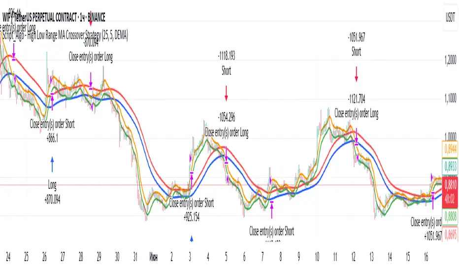
Script_Algo - Fibo Correction Strategy🔹 Core Concept
The strategy is built on combining Fibonacci retracement levels, candlestick pattern confirmation, and trend filtering for trade selection. It performs well on the 1-hour timeframe across many cryptocurrency pairs. Particularly on LINKUSDT over the past year and a half, despite the not very optimal 1:1 risk/reward ratio.
The logic is simple: after a strong impulse move, the price often retraces to key Fibonacci levels (specifically, the 61.8% level). If a confirming candlestick (pattern) appears at this moment, the strategy looks for an entry in the direction of the main trend.
🔹 Indicators Used in the Strategy
ATR (Average True Range) — Used to calculate the stop-loss and take-profit levels.
EMA (9 and 21) — Additional moving averages for assessing the direction of movement (not directly used in entry conditions, but the logic can be expanded to include them).
SMA (Trend Filter, 20 by default) — The trend direction filter. Trades are only opened in its direction.
Fibonacci Levels — The 61.8% retracement level is calculated based on the high and low of the previous candle.
🔹 Entry Conditions
🟢 Long (Buy):
Previous Candle:
Must be green (close higher than open).
Must have a body not smaller than a specified minimum.
The upper wick must not exceed 30% of the body size.
→ This filters out "weak" or "indecisive" candles.
Current Candle:
Price touches or breaches the Fibonacci 61.8% retracement level from the previous range.
Closes above this level.
Closes above the Trend Filter (SMA) line.
A position is opened only if there are no other open trades at the moment.
🔴 Short (Sell):
Previous Candle:
Must be red (close lower than open).
Must have a body not smaller than a specified minimum.
The lower wick must not exceed 30% of the body size.
Current Candle:
Price touches or breaches the Fibonacci 61.8% retracement level from the previous range.
Closes below this level.
Closes below the Trend Filter (SMA) line.
A trade is opened only if there are no other open positions.
🔹 Risk Management
Stop-Loss = ATR × multiplier (default is 5).
Take-Profit = ATR × the same multiplier.
Thus, the default risk/reward ratio is 1:1, but it can be easily adjusted by changing the coefficient. Although, strangely enough, this ratio has shown the best results on some assets on the 1-hour timeframe.
🔹 Chart Visualization
Fibonacci level for Long — Green line with circles.
Fibonacci level for Short — Red line with circles.
Trend Filter line (SMA) — Blue.
🔹 Strengths of the Strategy
✅ Utilizes a proven market pattern — retracement to the 61.8% level.
✅ Further filters entries using trend and candlestick patterns.
✅ Simple, transparent logic that is easy to expand (e.g., adding other Fib levels, an EMA filter, etc.).
🔹 Limitations
⚠️ Performs better in trending markets; can generate false signals during ranging (sideways) conditions.
⚠️ The fixed 1:1 risk/reward ratio is not always optimal and could be refined.
⚠️ Performance depends on the selected timeframe and ATR parameters.
📌 Summary:
The strategy seeks corrective entries in the direction of the trend, confirmed by candlestick patterns. It is versatile and can be applied to forex pairs, cryptocurrencies, and stocks.
⚠️ Not financial advice. Pay close attention to risk management to avoid blowing your account. The strategy is not repainting — I have personally verified it through real testing — but it may not necessarily replicate the same results in the future, as the market is constantly changing. Test it, profit, and good luck to everyone!
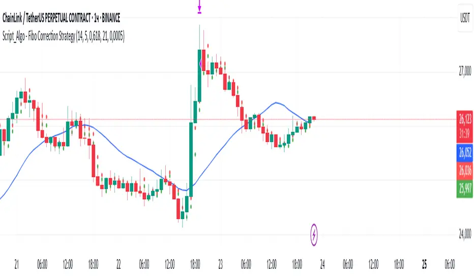
Markov Chain [3D] | FractalystWhat exactly is a Markov Chain?
This indicator uses a Markov Chain model to analyze, quantify, and visualize the transitions between market regimes (Bull, Bear, Neutral) on your chart. It dynamically detects these regimes in real-time, calculates transition probabilities, and displays them as animated 3D spheres and arrows, giving traders intuitive insight into current and future market conditions.
How does a Markov Chain work, and how should I read this spheres-and-arrows diagram?
Think of three weather modes: Sunny, Rainy, Cloudy.
Each sphere is one mode. The loop on a sphere means “stay the same next step” (e.g., Sunny again tomorrow).
The arrows leaving a sphere show where things usually go next if they change (e.g., Sunny moving to Cloudy).
Some paths matter more than others. A more prominent loop means the current mode tends to persist. A more prominent outgoing arrow means a change to that destination is the usual next step.
Direction isn’t symmetric: moving Sunny→Cloudy can behave differently than Cloudy→Sunny.
Now relabel the spheres to markets: Bull, Bear, Neutral.
Spheres: market regimes (uptrend, downtrend, range).
Self‑loop: tendency for the current regime to continue on the next bar.
Arrows: the most common next regime if a switch happens.
How to read: Start at the sphere that matches current bar state. If the loop stands out, expect continuation. If one outgoing path stands out, that switch is the typical next step. Opposite directions can differ (Bear→Neutral doesn’t have to match Neutral→Bear).
What states and transitions are shown?
The three market states visualized are:
Bullish (Bull): Upward or strong-market regime.
Bearish (Bear): Downward or weak-market regime.
Neutral: Sideways or range-bound regime.
Bidirectional animated arrows and probability labels show how likely the market is to move from one regime to another (e.g., Bull → Bear or Neutral → Bull).
How does the regime detection system work?
You can use either built-in price returns (based on adaptive Z-score normalization) or supply three custom indicators (such as volume, oscillators, etc.).
Values are statistically normalized (Z-scored) over a configurable lookback period.
The normalized outputs are classified into Bull, Bear, or Neutral zones.
If using three indicators, their regime signals are averaged and smoothed for robustness.
How are transition probabilities calculated?
On every confirmed bar, the algorithm tracks the sequence of detected market states, then builds a rolling window of transitions.
The code maintains a transition count matrix for all regime pairs (e.g., Bull → Bear).
Transition probabilities are extracted for each possible state change using Laplace smoothing for numerical stability, and frequently updated in real-time.
What is unique about the visualization?
3D animated spheres represent each regime and change visually when active.
Animated, bidirectional arrows reveal transition probabilities and allow you to see both dominant and less likely regime flows.
Particles (moving dots) animate along the arrows, enhancing the perception of regime flow direction and speed.
All elements dynamically update with each new price bar, providing a live market map in an intuitive, engaging format.
Can I use custom indicators for regime classification?
Yes! Enable the "Custom Indicators" switch and select any three chart series as inputs. These will be normalized and combined (each with equal weight), broadening the regime classification beyond just price-based movement.
What does the “Lookback Period” control?
Lookback Period (default: 100) sets how much historical data builds the probability matrix. Shorter periods adapt faster to regime changes but may be noisier. Longer periods are more stable but slower to adapt.
How is this different from a Hidden Markov Model (HMM)?
It sets the window for both regime detection and probability calculations. Lower values make the system more reactive, but potentially noisier. Higher values smooth estimates and make the system more robust.
How is this Markov Chain different from a Hidden Markov Model (HMM)?
Markov Chain (as here): All market regimes (Bull, Bear, Neutral) are directly observable on the chart. The transition matrix is built from actual detected regimes, keeping the model simple and interpretable.
Hidden Markov Model: The actual regimes are unobservable ("hidden") and must be inferred from market output or indicator "emissions" using statistical learning algorithms. HMMs are more complex, can capture more subtle structure, but are harder to visualize and require additional machine learning steps for training.
A standard Markov Chain models transitions between observable states using a simple transition matrix, while a Hidden Markov Model assumes the true states are hidden (latent) and must be inferred from observable “emissions” like price or volume data. In practical terms, a Markov Chain is transparent and easier to implement and interpret; an HMM is more expressive but requires statistical inference to estimate hidden states from data.
Markov Chain: states are observable; you directly count or estimate transition probabilities between visible states. This makes it simpler, faster, and easier to validate and tune.
HMM: states are hidden; you only observe emissions generated by those latent states. Learning involves machine learning/statistical algorithms (commonly Baum–Welch/EM for training and Viterbi for decoding) to infer both the transition dynamics and the most likely hidden state sequence from data.
How does the indicator avoid “repainting” or look-ahead bias?
All regime changes and matrix updates happen only on confirmed (closed) bars, so no future data is leaked, ensuring reliable real-time operation.
Are there practical tuning tips?
Tune the Lookback Period for your asset/timeframe: shorter for fast markets, longer for stability.
Use custom indicators if your asset has unique regime drivers.
Watch for rapid changes in transition probabilities as early warning of a possible regime shift.
Who is this indicator for?
Quants and quantitative researchers exploring probabilistic market modeling, especially those interested in regime-switching dynamics and Markov models.
Programmers and system developers who need a probabilistic regime filter for systematic and algorithmic backtesting:
The Markov Chain indicator is ideally suited for programmatic integration via its bias output (1 = Bull, 0 = Neutral, -1 = Bear).
Although the visualization is engaging, the core output is designed for automated, rules-based workflows—not for discretionary/manual trading decisions.
Developers can connect the indicator’s output directly to their Pine Script logic (using input.source()), allowing rapid and robust backtesting of regime-based strategies.
It acts as a plug-and-play regime filter: simply plug the bias output into your entry/exit logic, and you have a scientifically robust, probabilistically-derived signal for filtering, timing, position sizing, or risk regimes.
The MC's output is intentionally "trinary" (1/0/-1), focusing on clear regime states for unambiguous decision-making in code. If you require nuanced, multi-probability or soft-label state vectors, consider expanding the indicator or stacking it with a probability-weighted logic layer in your scripting.
Because it avoids subjectivity, this approach is optimal for systematic quants, algo developers building backtested, repeatable strategies based on probabilistic regime analysis.
What's the mathematical foundation behind this?
The mathematical foundation behind this Markov Chain indicator—and probabilistic regime detection in finance—draws from two principal models: the (standard) Markov Chain and the Hidden Markov Model (HMM).
How to use this indicator programmatically?
The Markov Chain indicator automatically exports a bias value (+1 for Bullish, -1 for Bearish, 0 for Neutral) as a plot visible in the Data Window. This allows you to integrate its regime signal into your own scripts and strategies for backtesting, automation, or live trading.
Step-by-Step Integration with Pine Script (input.source)
Add the Markov Chain indicator to your chart.
This must be done first, since your custom script will "pull" the bias signal from the indicator's plot.
In your strategy, create an input using input.source()
Example:
//@version=5
strategy("MC Bias Strategy Example")
mcBias = input.source(close, "MC Bias Source")
After saving, go to your script’s settings. For the “MC Bias Source” input, select the plot/output of the Markov Chain indicator (typically its bias plot).
Use the bias in your trading logic
Example (long only on Bull, flat otherwise):
if mcBias == 1
strategy.entry("Long", strategy.long)
else
strategy.close("Long")
For more advanced workflows, combine mcBias with additional filters or trailing stops.
How does this work behind-the-scenes?
TradingView’s input.source() lets you use any plot from another indicator as a real-time, “live” data feed in your own script (source).
The selected bias signal is available to your Pine code as a variable, enabling logical decisions based on regime (trend-following, mean-reversion, etc.).
This enables powerful strategy modularity : decouple regime detection from entry/exit logic, allowing fast experimentation without rewriting core signal code.
Integrating 45+ Indicators with Your Markov Chain — How & Why
The Enhanced Custom Indicators Export script exports a massive suite of over 45 technical indicators—ranging from classic momentum (RSI, MACD, Stochastic, etc.) to trend, volume, volatility, and oscillator tools—all pre-calculated, centered/scaled, and available as plots.
// Enhanced Custom Indicators Export - 45 Technical Indicators
// Comprehensive technical analysis suite for advanced market regime detection
//@version=6
indicator('Enhanced Custom Indicators Export | Fractalyst', shorttitle='Enhanced CI Export', overlay=false, scale=scale.right, max_labels_count=500, max_lines_count=500)
// |----- Input Parameters -----| //
momentum_group = "Momentum Indicators"
trend_group = "Trend Indicators"
volume_group = "Volume Indicators"
volatility_group = "Volatility Indicators"
oscillator_group = "Oscillator Indicators"
display_group = "Display Settings"
// Common lengths
length_14 = input.int(14, "Standard Length (14)", minval=1, maxval=100, group=momentum_group)
length_20 = input.int(20, "Medium Length (20)", minval=1, maxval=200, group=trend_group)
length_50 = input.int(50, "Long Length (50)", minval=1, maxval=200, group=trend_group)
// Display options
show_table = input.bool(true, "Show Values Table", group=display_group)
table_size = input.string("Small", "Table Size", options= , group=display_group)
// |----- MOMENTUM INDICATORS (15 indicators) -----| //
// 1. RSI (Relative Strength Index)
rsi_14 = ta.rsi(close, length_14)
rsi_centered = rsi_14 - 50
// 2. Stochastic Oscillator
stoch_k = ta.stoch(close, high, low, length_14)
stoch_d = ta.sma(stoch_k, 3)
stoch_centered = stoch_k - 50
// 3. Williams %R
williams_r = ta.stoch(close, high, low, length_14) - 100
// 4. MACD (Moving Average Convergence Divergence)
= ta.macd(close, 12, 26, 9)
// 5. Momentum (Rate of Change)
momentum = ta.mom(close, length_14)
momentum_pct = (momentum / close ) * 100
// 6. Rate of Change (ROC)
roc = ta.roc(close, length_14)
// 7. Commodity Channel Index (CCI)
cci = ta.cci(close, length_20)
// 8. Money Flow Index (MFI)
mfi = ta.mfi(close, length_14)
mfi_centered = mfi - 50
// 9. Awesome Oscillator (AO)
ao = ta.sma(hl2, 5) - ta.sma(hl2, 34)
// 10. Accelerator Oscillator (AC)
ac = ao - ta.sma(ao, 5)
// 11. Chande Momentum Oscillator (CMO)
cmo = ta.cmo(close, length_14)
// 12. Detrended Price Oscillator (DPO)
dpo = close - ta.sma(close, length_20)
// 13. Price Oscillator (PPO)
ppo = ta.sma(close, 12) - ta.sma(close, 26)
ppo_pct = (ppo / ta.sma(close, 26)) * 100
// 14. TRIX
trix_ema1 = ta.ema(close, length_14)
trix_ema2 = ta.ema(trix_ema1, length_14)
trix_ema3 = ta.ema(trix_ema2, length_14)
trix = ta.roc(trix_ema3, 1) * 10000
// 15. Klinger Oscillator
klinger = ta.ema(volume * (high + low + close) / 3, 34) - ta.ema(volume * (high + low + close) / 3, 55)
// 16. Fisher Transform
fisher_hl2 = 0.5 * (hl2 - ta.lowest(hl2, 10)) / (ta.highest(hl2, 10) - ta.lowest(hl2, 10)) - 0.25
fisher = 0.5 * math.log((1 + fisher_hl2) / (1 - fisher_hl2))
// 17. Stochastic RSI
stoch_rsi = ta.stoch(rsi_14, rsi_14, rsi_14, length_14)
stoch_rsi_centered = stoch_rsi - 50
// 18. Relative Vigor Index (RVI)
rvi_num = ta.swma(close - open)
rvi_den = ta.swma(high - low)
rvi = rvi_den != 0 ? rvi_num / rvi_den : 0
// 19. Balance of Power (BOP)
bop = (close - open) / (high - low)
// |----- TREND INDICATORS (10 indicators) -----| //
// 20. Simple Moving Average Momentum
sma_20 = ta.sma(close, length_20)
sma_momentum = ((close - sma_20) / sma_20) * 100
// 21. Exponential Moving Average Momentum
ema_20 = ta.ema(close, length_20)
ema_momentum = ((close - ema_20) / ema_20) * 100
// 22. Parabolic SAR
sar = ta.sar(0.02, 0.02, 0.2)
sar_trend = close > sar ? 1 : -1
// 23. Linear Regression Slope
lr_slope = ta.linreg(close, length_20, 0) - ta.linreg(close, length_20, 1)
// 24. Moving Average Convergence (MAC)
mac = ta.sma(close, 10) - ta.sma(close, 30)
// 25. Trend Intensity Index (TII)
tii_sum = 0.0
for i = 1 to length_20
tii_sum += close > close ? 1 : 0
tii = (tii_sum / length_20) * 100
// 26. Ichimoku Cloud Components
ichimoku_tenkan = (ta.highest(high, 9) + ta.lowest(low, 9)) / 2
ichimoku_kijun = (ta.highest(high, 26) + ta.lowest(low, 26)) / 2
ichimoku_signal = ichimoku_tenkan > ichimoku_kijun ? 1 : -1
// 27. MESA Adaptive Moving Average (MAMA)
mama_alpha = 2.0 / (length_20 + 1)
mama = ta.ema(close, length_20)
mama_momentum = ((close - mama) / mama) * 100
// 28. Zero Lag Exponential Moving Average (ZLEMA)
zlema_lag = math.round((length_20 - 1) / 2)
zlema_data = close + (close - close )
zlema = ta.ema(zlema_data, length_20)
zlema_momentum = ((close - zlema) / zlema) * 100
// |----- VOLUME INDICATORS (6 indicators) -----| //
// 29. On-Balance Volume (OBV)
obv = ta.obv
// 30. Volume Rate of Change (VROC)
vroc = ta.roc(volume, length_14)
// 31. Price Volume Trend (PVT)
pvt = ta.pvt
// 32. Negative Volume Index (NVI)
nvi = 0.0
nvi := volume < volume ? nvi + ((close - close ) / close ) * nvi : nvi
// 33. Positive Volume Index (PVI)
pvi = 0.0
pvi := volume > volume ? pvi + ((close - close ) / close ) * pvi : pvi
// 34. Volume Oscillator
vol_osc = ta.sma(volume, 5) - ta.sma(volume, 10)
// 35. Ease of Movement (EOM)
eom_distance = high - low
eom_box_height = volume / 1000000
eom = eom_box_height != 0 ? eom_distance / eom_box_height : 0
eom_sma = ta.sma(eom, length_14)
// 36. Force Index
force_index = volume * (close - close )
force_index_sma = ta.sma(force_index, length_14)
// |----- VOLATILITY INDICATORS (10 indicators) -----| //
// 37. Average True Range (ATR)
atr = ta.atr(length_14)
atr_pct = (atr / close) * 100
// 38. Bollinger Bands Position
bb_basis = ta.sma(close, length_20)
bb_dev = 2.0 * ta.stdev(close, length_20)
bb_upper = bb_basis + bb_dev
bb_lower = bb_basis - bb_dev
bb_position = bb_dev != 0 ? (close - bb_basis) / bb_dev : 0
bb_width = bb_dev != 0 ? (bb_upper - bb_lower) / bb_basis * 100 : 0
// 39. Keltner Channels Position
kc_basis = ta.ema(close, length_20)
kc_range = ta.ema(ta.tr, length_20)
kc_upper = kc_basis + (2.0 * kc_range)
kc_lower = kc_basis - (2.0 * kc_range)
kc_position = kc_range != 0 ? (close - kc_basis) / kc_range : 0
// 40. Donchian Channels Position
dc_upper = ta.highest(high, length_20)
dc_lower = ta.lowest(low, length_20)
dc_basis = (dc_upper + dc_lower) / 2
dc_position = (dc_upper - dc_lower) != 0 ? (close - dc_basis) / (dc_upper - dc_lower) : 0
// 41. Standard Deviation
std_dev = ta.stdev(close, length_20)
std_dev_pct = (std_dev / close) * 100
// 42. Relative Volatility Index (RVI)
rvi_up = ta.stdev(close > close ? close : 0, length_14)
rvi_down = ta.stdev(close < close ? close : 0, length_14)
rvi_total = rvi_up + rvi_down
rvi_volatility = rvi_total != 0 ? (rvi_up / rvi_total) * 100 : 50
// 43. Historical Volatility
hv_returns = math.log(close / close )
hv = ta.stdev(hv_returns, length_20) * math.sqrt(252) * 100
// 44. Garman-Klass Volatility
gk_vol = math.log(high/low) * math.log(high/low) - (2*math.log(2)-1) * math.log(close/open) * math.log(close/open)
gk_volatility = math.sqrt(ta.sma(gk_vol, length_20)) * 100
// 45. Parkinson Volatility
park_vol = math.log(high/low) * math.log(high/low)
parkinson = math.sqrt(ta.sma(park_vol, length_20) / (4 * math.log(2))) * 100
// 46. Rogers-Satchell Volatility
rs_vol = math.log(high/close) * math.log(high/open) + math.log(low/close) * math.log(low/open)
rogers_satchell = math.sqrt(ta.sma(rs_vol, length_20)) * 100
// |----- OSCILLATOR INDICATORS (5 indicators) -----| //
// 47. Elder Ray Index
elder_bull = high - ta.ema(close, 13)
elder_bear = low - ta.ema(close, 13)
elder_power = elder_bull + elder_bear
// 48. Schaff Trend Cycle (STC)
stc_macd = ta.ema(close, 23) - ta.ema(close, 50)
stc_k = ta.stoch(stc_macd, stc_macd, stc_macd, 10)
stc_d = ta.ema(stc_k, 3)
stc = ta.stoch(stc_d, stc_d, stc_d, 10)
// 49. Coppock Curve
coppock_roc1 = ta.roc(close, 14)
coppock_roc2 = ta.roc(close, 11)
coppock = ta.wma(coppock_roc1 + coppock_roc2, 10)
// 50. Know Sure Thing (KST)
kst_roc1 = ta.roc(close, 10)
kst_roc2 = ta.roc(close, 15)
kst_roc3 = ta.roc(close, 20)
kst_roc4 = ta.roc(close, 30)
kst = ta.sma(kst_roc1, 10) + 2*ta.sma(kst_roc2, 10) + 3*ta.sma(kst_roc3, 10) + 4*ta.sma(kst_roc4, 15)
// 51. Percentage Price Oscillator (PPO)
ppo_line = ((ta.ema(close, 12) - ta.ema(close, 26)) / ta.ema(close, 26)) * 100
ppo_signal = ta.ema(ppo_line, 9)
ppo_histogram = ppo_line - ppo_signal
// |----- PLOT MAIN INDICATORS -----| //
// Plot key momentum indicators
plot(rsi_centered, title="01_RSI_Centered", color=color.purple, linewidth=1)
plot(stoch_centered, title="02_Stoch_Centered", color=color.blue, linewidth=1)
plot(williams_r, title="03_Williams_R", color=color.red, linewidth=1)
plot(macd_histogram, title="04_MACD_Histogram", color=color.orange, linewidth=1)
plot(cci, title="05_CCI", color=color.green, linewidth=1)
// Plot trend indicators
plot(sma_momentum, title="06_SMA_Momentum", color=color.navy, linewidth=1)
plot(ema_momentum, title="07_EMA_Momentum", color=color.maroon, linewidth=1)
plot(sar_trend, title="08_SAR_Trend", color=color.teal, linewidth=1)
plot(lr_slope, title="09_LR_Slope", color=color.lime, linewidth=1)
plot(mac, title="10_MAC", color=color.fuchsia, linewidth=1)
// Plot volatility indicators
plot(atr_pct, title="11_ATR_Pct", color=color.yellow, linewidth=1)
plot(bb_position, title="12_BB_Position", color=color.aqua, linewidth=1)
plot(kc_position, title="13_KC_Position", color=color.olive, linewidth=1)
plot(std_dev_pct, title="14_StdDev_Pct", color=color.silver, linewidth=1)
plot(bb_width, title="15_BB_Width", color=color.gray, linewidth=1)
// Plot volume indicators
plot(vroc, title="16_VROC", color=color.blue, linewidth=1)
plot(eom_sma, title="17_EOM", color=color.red, linewidth=1)
plot(vol_osc, title="18_Vol_Osc", color=color.green, linewidth=1)
plot(force_index_sma, title="19_Force_Index", color=color.orange, linewidth=1)
plot(obv, title="20_OBV", color=color.purple, linewidth=1)
// Plot additional oscillators
plot(ao, title="21_Awesome_Osc", color=color.navy, linewidth=1)
plot(cmo, title="22_CMO", color=color.maroon, linewidth=1)
plot(dpo, title="23_DPO", color=color.teal, linewidth=1)
plot(trix, title="24_TRIX", color=color.lime, linewidth=1)
plot(fisher, title="25_Fisher", color=color.fuchsia, linewidth=1)
// Plot more momentum indicators
plot(mfi_centered, title="26_MFI_Centered", color=color.yellow, linewidth=1)
plot(ac, title="27_AC", color=color.aqua, linewidth=1)
plot(ppo_pct, title="28_PPO_Pct", color=color.olive, linewidth=1)
plot(stoch_rsi_centered, title="29_StochRSI_Centered", color=color.silver, linewidth=1)
plot(klinger, title="30_Klinger", color=color.gray, linewidth=1)
// Plot trend continuation
plot(tii, title="31_TII", color=color.blue, linewidth=1)
plot(ichimoku_signal, title="32_Ichimoku_Signal", color=color.red, linewidth=1)
plot(mama_momentum, title="33_MAMA_Momentum", color=color.green, linewidth=1)
plot(zlema_momentum, title="34_ZLEMA_Momentum", color=color.orange, linewidth=1)
plot(bop, title="35_BOP", color=color.purple, linewidth=1)
// Plot volume continuation
plot(nvi, title="36_NVI", color=color.navy, linewidth=1)
plot(pvi, title="37_PVI", color=color.maroon, linewidth=1)
plot(momentum_pct, title="38_Momentum_Pct", color=color.teal, linewidth=1)
plot(roc, title="39_ROC", color=color.lime, linewidth=1)
plot(rvi, title="40_RVI", color=color.fuchsia, linewidth=1)
// Plot volatility continuation
plot(dc_position, title="41_DC_Position", color=color.yellow, linewidth=1)
plot(rvi_volatility, title="42_RVI_Volatility", color=color.aqua, linewidth=1)
plot(hv, title="43_Historical_Vol", color=color.olive, linewidth=1)
plot(gk_volatility, title="44_GK_Volatility", color=color.silver, linewidth=1)
plot(parkinson, title="45_Parkinson_Vol", color=color.gray, linewidth=1)
// Plot final oscillators
plot(rogers_satchell, title="46_RS_Volatility", color=color.blue, linewidth=1)
plot(elder_power, title="47_Elder_Power", color=color.red, linewidth=1)
plot(stc, title="48_STC", color=color.green, linewidth=1)
plot(coppock, title="49_Coppock", color=color.orange, linewidth=1)
plot(kst, title="50_KST", color=color.purple, linewidth=1)
// Plot final indicators
plot(ppo_histogram, title="51_PPO_Histogram", color=color.navy, linewidth=1)
plot(pvt, title="52_PVT", color=color.maroon, linewidth=1)
// |----- Reference Lines -----| //
hline(0, "Zero Line", color=color.gray, linestyle=hline.style_dashed, linewidth=1)
hline(50, "Midline", color=color.gray, linestyle=hline.style_dotted, linewidth=1)
hline(-50, "Lower Midline", color=color.gray, linestyle=hline.style_dotted, linewidth=1)
hline(25, "Upper Threshold", color=color.gray, linestyle=hline.style_dotted, linewidth=1)
hline(-25, "Lower Threshold", color=color.gray, linestyle=hline.style_dotted, linewidth=1)
// |----- Enhanced Information Table -----| //
if show_table and barstate.islast
table_position = position.top_right
table_text_size = table_size == "Tiny" ? size.tiny : table_size == "Small" ? size.small : size.normal
var table info_table = table.new(table_position, 3, 18, bgcolor=color.new(color.white, 85), border_width=1, border_color=color.gray)
// Headers
table.cell(info_table, 0, 0, 'Category', text_color=color.black, text_size=table_text_size, bgcolor=color.new(color.blue, 70))
table.cell(info_table, 1, 0, 'Indicator', text_color=color.black, text_size=table_text_size, bgcolor=color.new(color.blue, 70))
table.cell(info_table, 2, 0, 'Value', text_color=color.black, text_size=table_text_size, bgcolor=color.new(color.blue, 70))
// Key Momentum Indicators
table.cell(info_table, 0, 1, 'MOMENTUM', text_color=color.purple, text_size=table_text_size, bgcolor=color.new(color.purple, 90))
table.cell(info_table, 1, 1, 'RSI Centered', text_color=color.purple, text_size=table_text_size)
table.cell(info_table, 2, 1, str.tostring(rsi_centered, '0.00'), text_color=color.purple, text_size=table_text_size)
table.cell(info_table, 0, 2, '', text_color=color.blue, text_size=table_text_size)
table.cell(info_table, 1, 2, 'Stoch Centered', text_color=color.blue, text_size=table_text_size)
table.cell(info_table, 2, 2, str.tostring(stoch_centered, '0.00'), text_color=color.blue, text_size=table_text_size)
table.cell(info_table, 0, 3, '', text_color=color.red, text_size=table_text_size)
table.cell(info_table, 1, 3, 'Williams %R', text_color=color.red, text_size=table_text_size)
table.cell(info_table, 2, 3, str.tostring(williams_r, '0.00'), text_color=color.red, text_size=table_text_size)
table.cell(info_table, 0, 4, '', text_color=color.orange, text_size=table_text_size)
table.cell(info_table, 1, 4, 'MACD Histogram', text_color=color.orange, text_size=table_text_size)
table.cell(info_table, 2, 4, str.tostring(macd_histogram, '0.000'), text_color=color.orange, text_size=table_text_size)
table.cell(info_table, 0, 5, '', text_color=color.green, text_size=table_text_size)
table.cell(info_table, 1, 5, 'CCI', text_color=color.green, text_size=table_text_size)
table.cell(info_table, 2, 5, str.tostring(cci, '0.00'), text_color=color.green, text_size=table_text_size)
// Key Trend Indicators
table.cell(info_table, 0, 6, 'TREND', text_color=color.navy, text_size=table_text_size, bgcolor=color.new(color.navy, 90))
table.cell(info_table, 1, 6, 'SMA Momentum %', text_color=color.navy, text_size=table_text_size)
table.cell(info_table, 2, 6, str.tostring(sma_momentum, '0.00'), text_color=color.navy, text_size=table_text_size)
table.cell(info_table, 0, 7, '', text_color=color.maroon, text_size=table_text_size)
table.cell(info_table, 1, 7, 'EMA Momentum %', text_color=color.maroon, text_size=table_text_size)
table.cell(info_table, 2, 7, str.tostring(ema_momentum, '0.00'), text_color=color.maroon, text_size=table_text_size)
table.cell(info_table, 0, 8, '', text_color=color.teal, text_size=table_text_size)
table.cell(info_table, 1, 8, 'SAR Trend', text_color=color.teal, text_size=table_text_size)
table.cell(info_table, 2, 8, str.tostring(sar_trend, '0'), text_color=color.teal, text_size=table_text_size)
table.cell(info_table, 0, 9, '', text_color=color.lime, text_size=table_text_size)
table.cell(info_table, 1, 9, 'Linear Regression', text_color=color.lime, text_size=table_text_size)
table.cell(info_table, 2, 9, str.tostring(lr_slope, '0.000'), text_color=color.lime, text_size=table_text_size)
// Key Volatility Indicators
table.cell(info_table, 0, 10, 'VOLATILITY', text_color=color.yellow, text_size=table_text_size, bgcolor=color.new(color.yellow, 90))
table.cell(info_table, 1, 10, 'ATR %', text_color=color.yellow, text_size=table_text_size)
table.cell(info_table, 2, 10, str.tostring(atr_pct, '0.00'), text_color=color.yellow, text_size=table_text_size)
table.cell(info_table, 0, 11, '', text_color=color.aqua, text_size=table_text_size)
table.cell(info_table, 1, 11, 'BB Position', text_color=color.aqua, text_size=table_text_size)
table.cell(info_table, 2, 11, str.tostring(bb_position, '0.00'), text_color=color.aqua, text_size=table_text_size)
table.cell(info_table, 0, 12, '', text_color=color.olive, text_size=table_text_size)
table.cell(info_table, 1, 12, 'KC Position', text_color=color.olive, text_size=table_text_size)
table.cell(info_table, 2, 12, str.tostring(kc_position, '0.00'), text_color=color.olive, text_size=table_text_size)
// Key Volume Indicators
table.cell(info_table, 0, 13, 'VOLUME', text_color=color.blue, text_size=table_text_size, bgcolor=color.new(color.blue, 90))
table.cell(info_table, 1, 13, 'Volume ROC', text_color=color.blue, text_size=table_text_size)
table.cell(info_table, 2, 13, str.tostring(vroc, '0.00'), text_color=color.blue, text_size=table_text_size)
table.cell(info_table, 0, 14, '', text_color=color.red, text_size=table_text_size)
table.cell(info_table, 1, 14, 'EOM', text_color=color.red, text_size=table_text_size)
table.cell(info_table, 2, 14, str.tostring(eom_sma, '0.000'), text_color=color.red, text_size=table_text_size)
// Key Oscillators
table.cell(info_table, 0, 15, 'OSCILLATORS', text_color=color.purple, text_size=table_text_size, bgcolor=color.new(color.purple, 90))
table.cell(info_table, 1, 15, 'Awesome Osc', text_color=color.blue, text_size=table_text_size)
table.cell(info_table, 2, 15, str.tostring(ao, '0.000'), text_color=color.blue, text_size=table_text_size)
table.cell(info_table, 0, 16, '', text_color=color.red, text_size=table_text_size)
table.cell(info_table, 1, 16, 'Fisher Transform', text_color=color.red, text_size=table_text_size)
table.cell(info_table, 2, 16, str.tostring(fisher, '0.000'), text_color=color.red, text_size=table_text_size)
// Summary Statistics
table.cell(info_table, 0, 17, 'SUMMARY', text_color=color.black, text_size=table_text_size, bgcolor=color.new(color.gray, 70))
table.cell(info_table, 1, 17, 'Total Indicators: 52', text_color=color.black, text_size=table_text_size)
regime_color = rsi_centered > 10 ? color.green : rsi_centered < -10 ? color.red : color.gray
regime_text = rsi_centered > 10 ? "BULLISH" : rsi_centered < -10 ? "BEARISH" : "NEUTRAL"
table.cell(info_table, 2, 17, regime_text, text_color=regime_color, text_size=table_text_size)
This makes it the perfect “indicator backbone” for quantitative and systematic traders who want to prototype, combine, and test new regime detection models—especially in combination with the Markov Chain indicator.
How to use this script with the Markov Chain for research and backtesting:
Add the Enhanced Indicator Export to your chart.
Every calculated indicator is available as an individual data stream.
Connect the indicator(s) you want as custom input(s) to the Markov Chain’s “Custom Indicators” option.
In the Markov Chain indicator’s settings, turn ON the custom indicator mode.
For each of the three custom indicator inputs, select the exported plot from the Enhanced Export script—the menu lists all 45+ signals by name.
This creates a powerful, modular regime-detection engine where you can mix-and-match momentum, trend, volume, or custom combinations for advanced filtering.
Backtest regime logic directly.
Once you’ve connected your chosen indicators, the Markov Chain script performs regime detection (Bull/Neutral/Bear) based on your selected features—not just price returns.
The regime detection is robust, automatically normalized (using Z-score), and outputs bias (1, -1, 0) for plug-and-play integration.
Export the regime bias for programmatic use.
As described above, use input.source() in your Pine Script strategy or system and link the bias output.
You can now filter signals, control trade direction/size, or design pairs-trading that respect true, indicator-driven market regimes.
With this framework, you’re not limited to static or simplistic regime filters. You can rigorously define, test, and refine what “market regime” means for your strategies—using the technical features that matter most to you.
Optimize your signal generation by backtesting across a universe of meaningful indicator blends.
Enhance risk management with objective, real-time regime boundaries.
Accelerate your research: iterate quickly, swap indicator components, and see results with minimal code changes.
Automate multi-asset or pairs-trading by integrating regime context directly into strategy logic.
Add both scripts to your chart, connect your preferred features, and start investigating your best regime-based trades—entirely within the TradingView ecosystem.
References & Further Reading
Ang, A., & Bekaert, G. (2002). “Regime Switches in Interest Rates.” Journal of Business & Economic Statistics, 20(2), 163–182.
Hamilton, J. D. (1989). “A New Approach to the Economic Analysis of Nonstationary Time Series and the Business Cycle.” Econometrica, 57(2), 357–384.
Markov, A. A. (1906). "Extension of the Limit Theorems of Probability Theory to a Sum of Variables Connected in a Chain." The Notes of the Imperial Academy of Sciences of St. Petersburg.
Guidolin, M., & Timmermann, A. (2007). “Asset Allocation under Multivariate Regime Switching.” Journal of Economic Dynamics and Control, 31(11), 3503–3544.
Murphy, J. J. (1999). Technical Analysis of the Financial Markets. New York Institute of Finance.
Brock, W., Lakonishok, J., & LeBaron, B. (1992). “Simple Technical Trading Rules and the Stochastic Properties of Stock Returns.” Journal of Finance, 47(5), 1731–1764.
Zucchini, W., MacDonald, I. L., & Langrock, R. (2017). Hidden Markov Models for Time Series: An Introduction Using R (2nd ed.). Chapman and Hall/CRC.
On Quantitative Finance and Markov Models:
Lo, A. W., & Hasanhodzic, J. (2009). The Heretics of Finance: Conversations with Leading Practitioners of Technical Analysis. Bloomberg Press.
Patterson, S. (2016). The Man Who Solved the Market: How Jim Simons Launched the Quant Revolution. Penguin Press.
TradingView Pine Script Documentation: www.tradingview.com
TradingView Blog: “Use an Input From Another Indicator With Your Strategy” www.tradingview.com
GeeksforGeeks: “What is the Difference Between Markov Chains and Hidden Markov Models?” www.geeksforgeeks.org
What makes this indicator original and unique?
- On‑chart, real‑time Markov. The chain is drawn directly on your chart. You see the current regime, its tendency to stay (self‑loop), and the usual next step (arrows) as bars confirm.
- Source‑agnostic by design. The engine runs on any series you select via input.source() — price, your own oscillator, a composite score, anything you compute in the script.
- Automatic normalization + regime mapping. Different inputs live on different scales. The script standardizes your chosen source and maps it into clear regimes (e.g., Bull / Bear / Neutral) without you micromanaging thresholds each time.
- Rolling, bar‑by‑bar learning. Transition tendencies are computed from a rolling window of confirmed bars. What you see is exactly what the market did in that window.
- Fast experimentation. Switch the source, adjust the window, and the Markov view updates instantly. It’s a rapid way to test ideas and feel regime persistence/switch behavior.
Integrate your own signals (using input.source())
- In settings, choose the Source . This is powered by input.source() .
- Feed it price, an indicator you compute inside the script, or a custom composite series.
- The script will automatically normalize that series and process it through the Markov engine, mapping it to regimes and updating the on‑chart spheres/arrows in real time.
Credits:
Deep gratitude to @RicardoSantos for both the foundational Markov chain processing engine and inspiring open-source contributions, which made advanced probabilistic market modeling accessible to the TradingView community.
Special thanks to @Alien_Algorithms for the innovative and visually stunning 3D sphere logic that powers the indicator’s animated, regime-based visualization.
Disclaimer
This tool summarizes recent behavior. It is not financial advice and not a guarantee of future results.

Order Blocks v2Order Blocks v2 – Smart OB Detection with Time & FVG Filters
Order Blocks v2 is an advanced tool designed to identify potential institutional footprints in the market by dynamically plotting bullish and bearish order blocks.
This indicator refines classic OB logic by combining:
Fractal-based break conditions
Time-level filtering (Power of 3)
Optional Fair Value Gap (FVG) confirmation
Real-time plotting and auto-invalidation
Perfect for traders using ICT, Smart Money, or algorithmic timing models like Hopplipka.
🧠 What the indicator does
Detects order blocks after break of bullish/bearish fractals
Supports 3-bar or 5-bar fractal structures
Allows OB detection based on close breaks or high/low breaks
Optionally confirms OBs only if followed by a Fair Value Gap within N candles
Filters OBs based on specific time levels (3, 7, 11, 14) — core anchors in many algorithmic models
Automatically deletes invalidated OBs once price closes through the zone
⚙️ How it works
The indicator:
Tracks local fractal highs/lows
Once a fractal is broken by price, it backtracks to identify the best OB candle (highest bullish or lowest bearish)
Validates the level by checking:
OB type logic (close or HL break)
Time stamp match with algorithmic time anchors (e.g. 3, 7, 11, 14 – known from the Power of 3 concept)
Optional FVG confirmation after OB
Plots OB zones as lines (body or wick-based) and removes them if invalidated by a candle close
This ensures traders see only valid, active levels — removing noise from broken or out-of-context zones.
🔧 Customization
Choose 3-bar or 5-bar fractals
OB detection type: close break or HL break
Enable/disable OBs only on times 3, 7, 11, 14 (Hopplipka style)
Optional: require nearby FVG for validation
Line style: solid, dashed, or dotted
Adjust OB length, width, color, and use body or wick for OB height
🚀 How to use it
Add the script to your chart
Choose your preferred OB detection mode and filters
Use plotted OB zones to:
Anticipate price rejections and reversals
Validate Smart Money or ICT-based entry zones
Align setups with algorithmic time sequences (3, 7, 11, 14)
Filter out invalid OBs automatically, keeping your chart clean
The tool is useful on any timeframe but performs best when combined with a liquidity-based or time-anchored trading model.
💡 What makes it original
Combines fractal logic with OB confirmation and time anchors
Implements time-based filtering inspired by Hopplipka’s interpretation of the "Power of 3"
Allows OB validation via optional FVG follow-up — rarely available in public indicators
Auto-cleans invalidated OBs to reduce clutter
Designed to reflect market structure logic used by institutions and algorithms
💬 Why it’s worth using
Order Blocks v2 simplifies one of the most nuanced parts of SMC: identifying clean and high-probability OBs.
It removes subjectivity, adds clear timing logic, and integrates optional confluence tools — like FVG.
For traders serious about algorithmic-level structure and clean setups, this tool delivers both logic and clarity.
⚠️ Important
This indicator:
Is not a signal generator or financial advice tool
Is intended for experienced traders using OB/SMC/time-based logic
Does not predict market direction — it provides visual structural levels only