Debugging

Introduction

TradingView’s close integration between the Pine Editor and the Supercharts interface enables efficient, interactive debugging of Pine Script® code. Pine scripts can create dynamic outputs in multiple locations, on and off the chart. Programmers can use these outputs to validate their scripts’ behaviors and ensure everything works as expected.

Understanding the most effective tools and methods for inspecting a script helps programmers quickly find and fix potential problems in their code, which improves the overall coding experience. This page explains the script outputs that are the most useful for debugging, along with helpful tips and techniques.

Common debug outputs

Pine scripts can create outputs in several ways, each of which has different advantages. While programmers can use any of them to debug their code, some outputs are more optimal for debugging than others.

The functions in the log.* namespace log interactive messages in the Pine Logs pane. These logging functions are the most convenient and flexible tools for debugging Pine code. Scripts can call log.*() functions on any execution from global or local scopes, enabling programmers to analyze historical and realtime script behaviors in depth with minimal code, for example:

Pine drawings display visuals in the main chart pane or the script’s separate pane. Although they do not output results in other locations, such as the Data Window or Pine Logs pane, drawings provide convenient ways to visualize a script’s data and logic within global or local scopes. Labels are the most flexible drawings for debugging, because they can display colored shapes with formatted text and tooltips at any available chart location, for example:

The plot*() functions can help to debug numeric values, conditions, and colors from a script’s global scope. They can output results in up to four locations: the main chart pane or the script’s pane, the status line, the price scale, and the Data Window. The display on the chart provides a quick view of the series’ history, and the numbers in the other output locations show calculated information for specific bars:

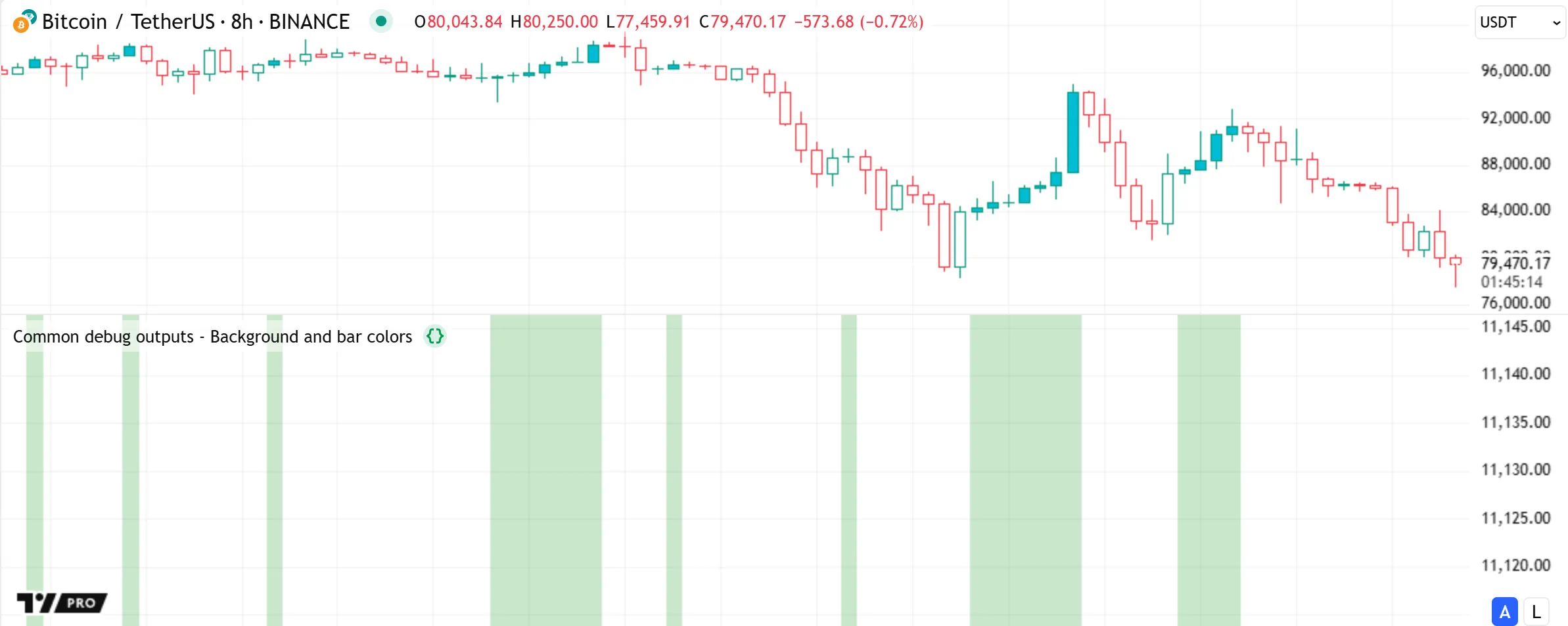
The bgcolor() function displays colors in the background of the main chart pane or the script’s pane. The barcolor() function colors the main chart’s bars or candles. Although these outputs are less flexible than Pine Logs, drawings, and plots, they provide a quick way to inspect calculated colors and visualize conditions from the global scope:

Programmers can use any of these outputs individually or in combination to debug their scripts, depending on the data types and structures that require inspection. See the sections below for detailed information about these outputs and various debugging techniques.

Pine Logs

Pine Logs are interactive, user-defined messages that scripts can create from within global or local scopes at any point during code executions on the chart’s dataset or requested datasets. They provide a simple, powerful way for programmers to inspect a script’s calculations, logic, and execution flow with human-readable text. Using Pine Logs is the primary, most universal technique for debugging Pine Script code.

Pine Logs do not appear on the chart or in the Data Window. Instead, scripts print logged messages with prefixed date and time information in the dedicated Pine Logs pane. The inspection and filtering options in the Pine Logs pane help users analyze and navigate logs efficiently.

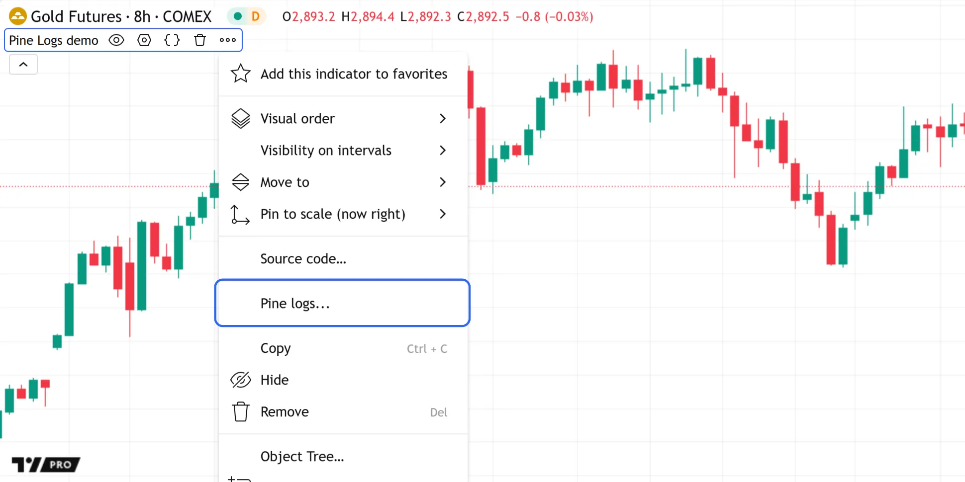
To access the pane, select “Pine Logs” from the Pine Editor’s “More” menu or from the “More” menu in the status line of a script on the chart that uses the log.*() functions:

Creating logs

Scripts create Pine Logs by calling the functions in the log.* namespace: log.info(), log.warning(), or log.error(). All these logging functions have the following two signatures:

log.*(message) → void
log.*(formatString, arg0, arg1, ...) → void

Where:

• The first overload prints the specified “string” message in the Pine Logs pane.
• The second overload creates a formatted string based on its formatString and additional arguments, similar to str.format(), then displays the resulting text inside the pane.

Each log.*() function has a different logging level, allowing programmers to categorize the messages shown in the Pine Logs pane:

• The log.info() function creates a message with the “info” level (gray text).
• The log.warning() function creates a message with the “warning” level (orange text).
• The log.error() function creates a message with the “error” level (red text).

This simple script demonstrates the difference between all three log.*() functions. It calls log.info(), log.warning(), and log.error() on the first chart bar to print the values of three literal strings in the Pine Logs pane:

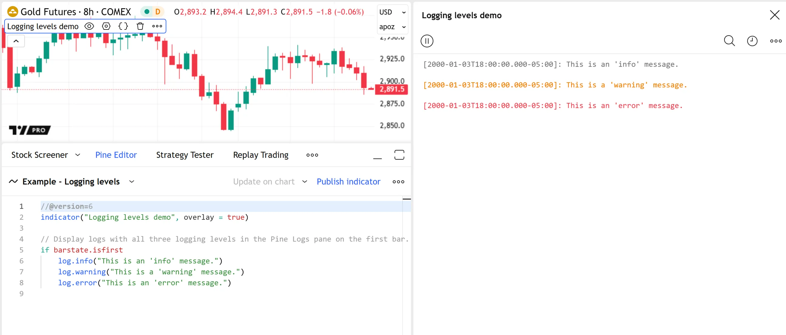
Note that:

• The Pine Logs pane can filter messages by their logging level using the menu accessible from the rightmost icon above the logs. See the Filtering logs section to learn more.

Scripts can generate logs at any point during their executions, allowing programmers to track information from historical bars, and monitor script behaviors on open realtime bars.

During historical executions, scripts log a new message once for each log.*() call on any bar. During realtime executions, scripts can call the log.*() functions to log messages for any available tick, regardless of whether the bar is confirmed. The logs created on realtime ticks are not subject to rollback. All logs remain available in the Pine Logs pane until the script restarts.

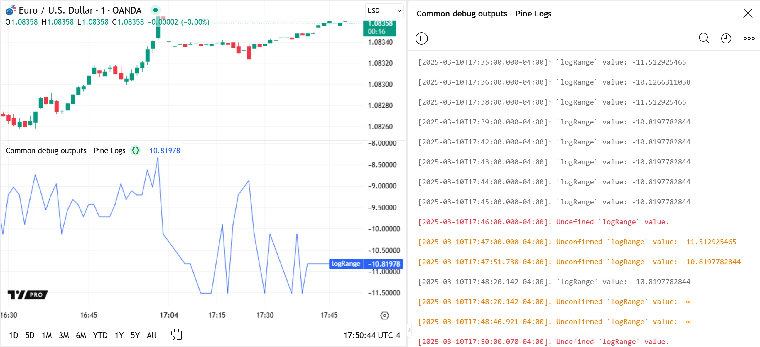
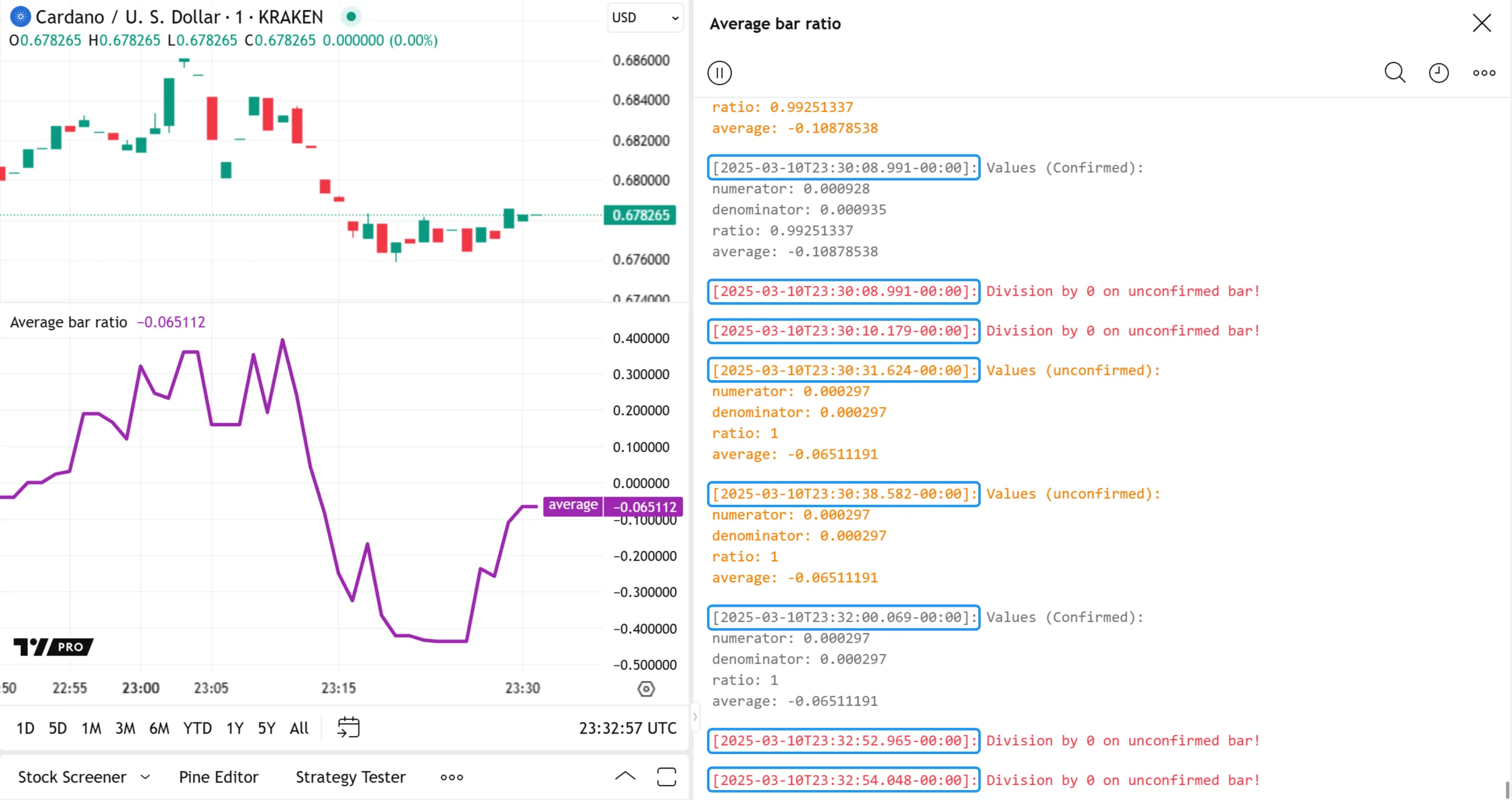
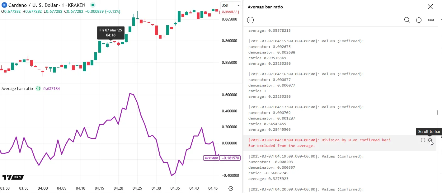
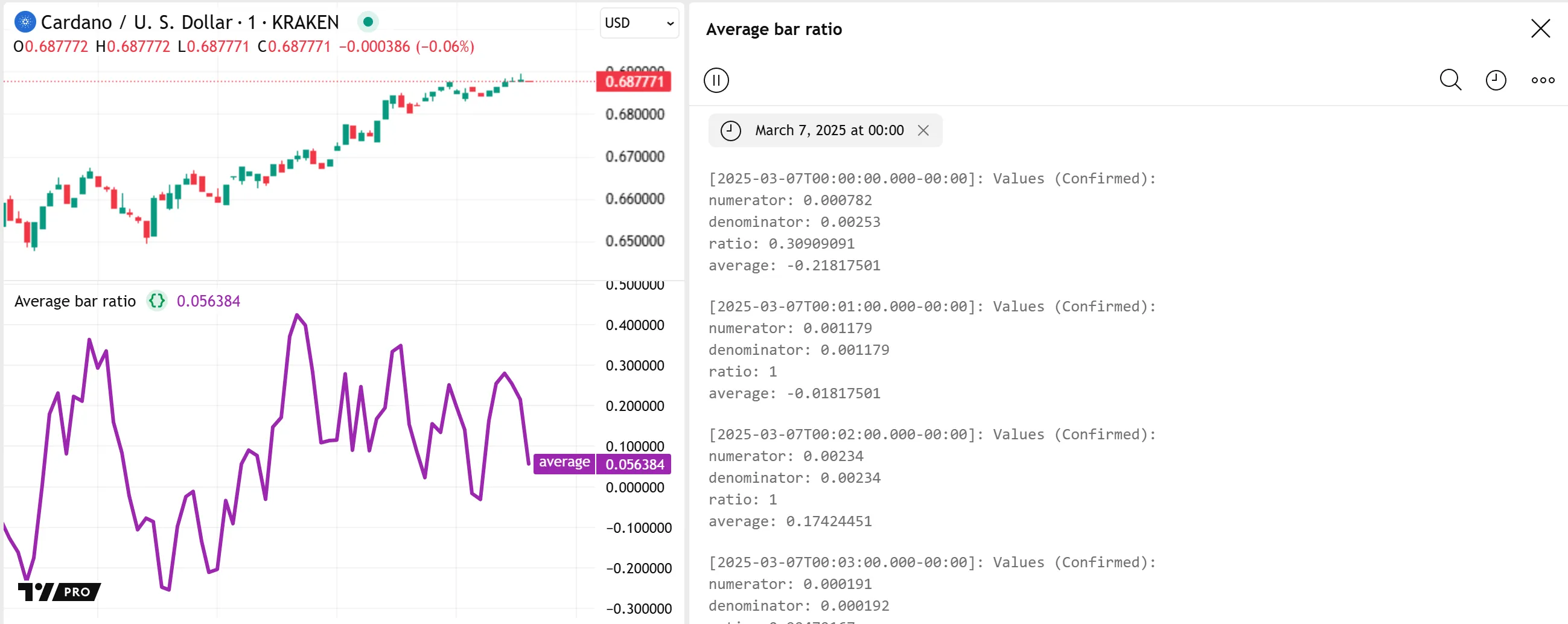
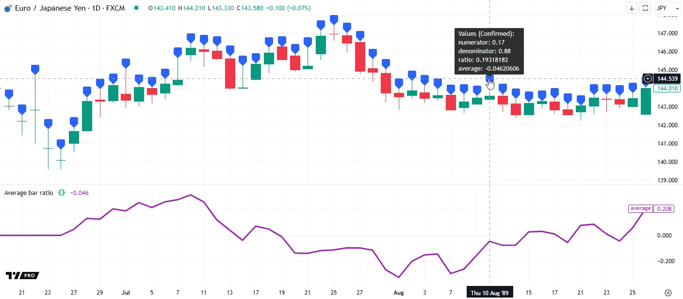
The example script below calculates the average ratio of each bar’s close - open value to its high - low range. When the range is nonzero, the script prints the values of the calculation’s variables in the Pine Logs pane using log.info() if the bar is confirmed or log.warning() if the bar is still open (unconfirmed). If the bar’s range is zero, making the calculated ratio undefined, the script logs an “error” message using log.error():

Note that:

• Programmers can use barstate.isconfirmed in the conditions that trigger log.*() calls to allow logs for any realtime bar only once, on its closing tick, as shown in the example code.
• Users can pause realtime logs by selecting the “Disable logging” button at the top of the Pine Logs pane.
• Allowing logging on any tick of an open bar can result in a large number of logged messages over time. Therefore, we recommend including unique information in the messages or using different logging levels for easy filtering from the Pine Logs pane.
• The Pine Logs pane can display the most recent 10,000 logs for historical bars. If a programmer needs to view earlier logs, they can add logic in the code to filter specific log.*() calls. See the Custom code filters section for an example.

The following sections use the example script above to demonstrate the Pine Logs pane’s log inspection and filtering features.

Inspecting logs

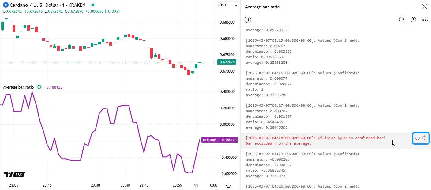
When a script generates a log by calling any log.*() function call, the Pine Logs pane automatically prefixes the logged message with an ISO 8601 timestamp representing the log’s assigned time, expressed in the chart’s time zone. The timestamp prefixed to a log on a historical bar represents the bar’s opening time, whereas the timestamp for a realtime log represents the system time of the log event:

Additionally, each log includes “Source code” and “Scroll to bar” options, which appear when hovering over the message in the Pine Logs pane. These features provide convenient ways for users to inspect and verify a log’s conditions:

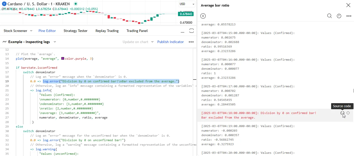
The “Source code” option opens the script in the Pine Editor and highlights the code line containing the specific log.*() call that triggered the log event:

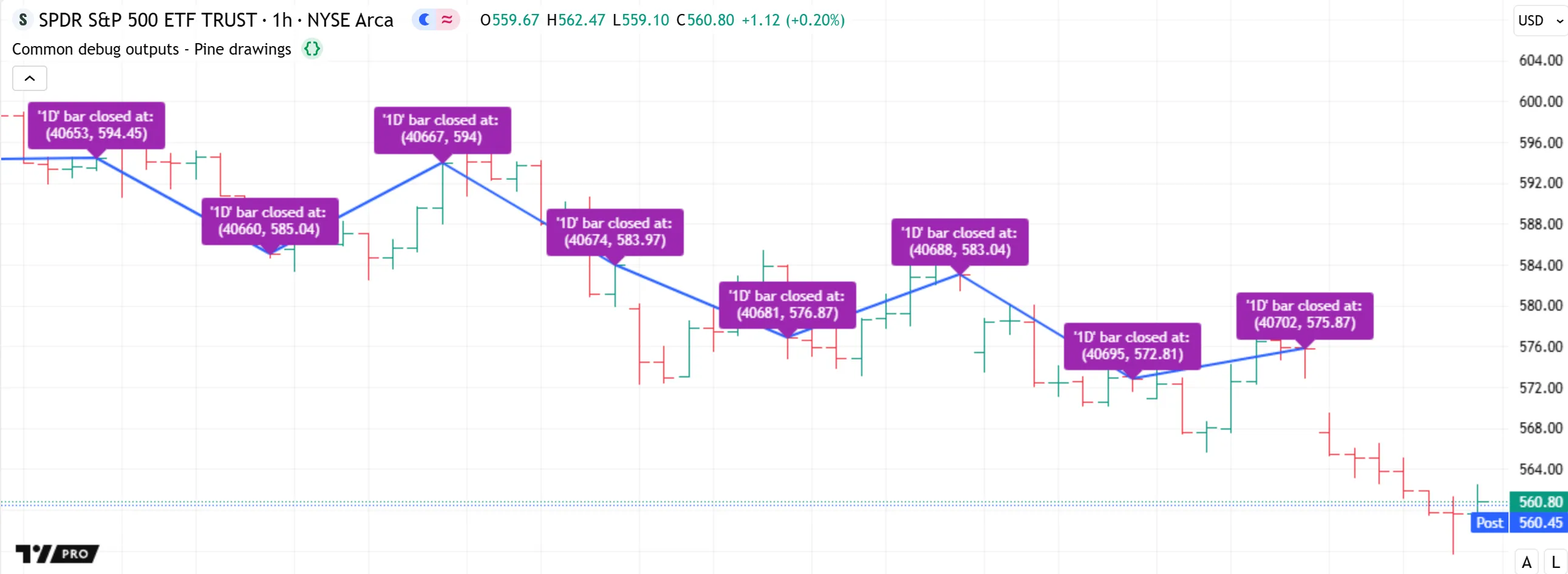
The “Scroll to bar” option navigates the chart to the bar where the log.*() call occurred, then displays a temporary label above the bar, containing its date and time information:

Note that:

• The label’s time information depends on the chart’s timeframe. For example, the label on a “1D” chart contains only the weekday and date, whereas the label on an intraday chart also includes the time of day.

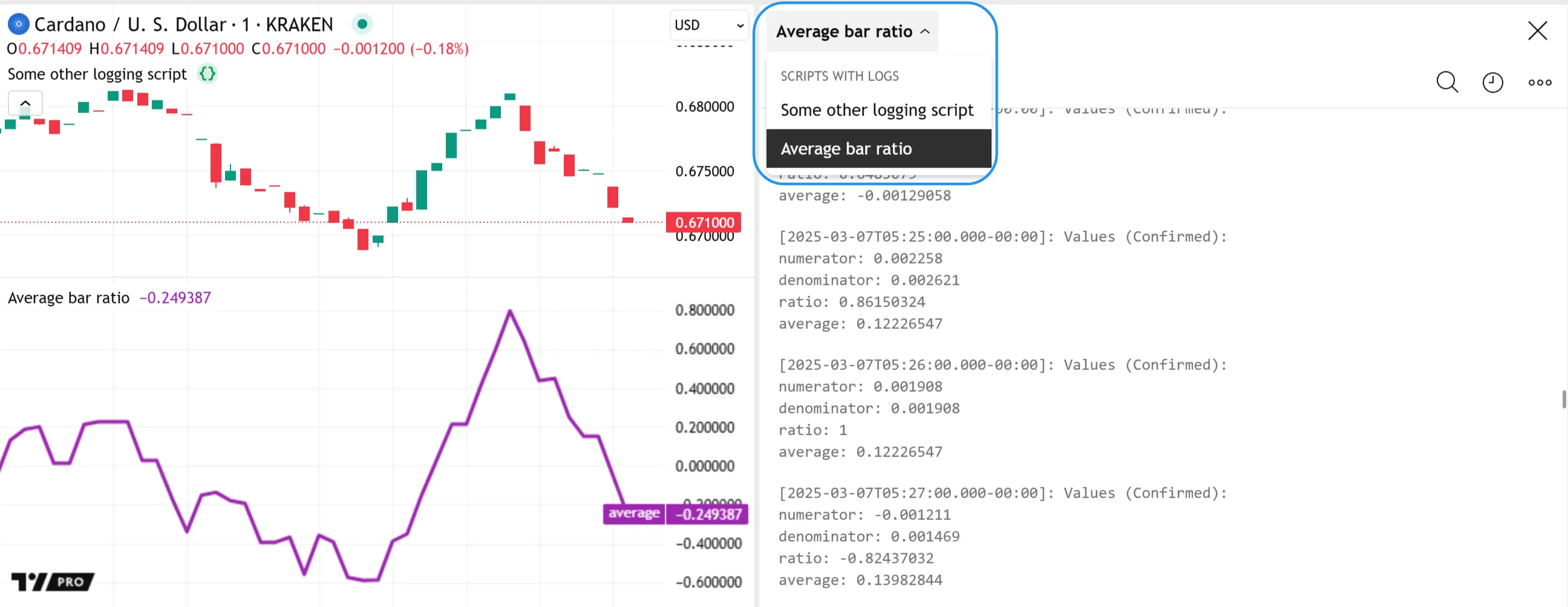
It’s important to note that every script on the chart that generates logs maintains an independent log history. The Pine Logs pane shows logs for only one script at a time. To inspect the logs from a specific script when multiple are on the chart, select its title from the dropdown menu at the top of the pane:

Filtering logs

The Pine Logs pane displays up to 10,000 logged messages from script executions on historical bars. It then appends a new log for each log.*() call executed on any realtime tick.

To help users navigate high volumes of logs efficiently, the pane includes filters that isolate logs based on logging level, start date and time, or search queries. Users can apply these log filters individually or in combination to show only the messages that meet specific criteria. The filters are accessible from the icons below the “x” in the top-right portion of the pane:

For custom filtering options, programmers can use conditional logic to activate specific log.*() calls selectively across a script’s executions. See the Custom code filters section below to learn more.

Logging level

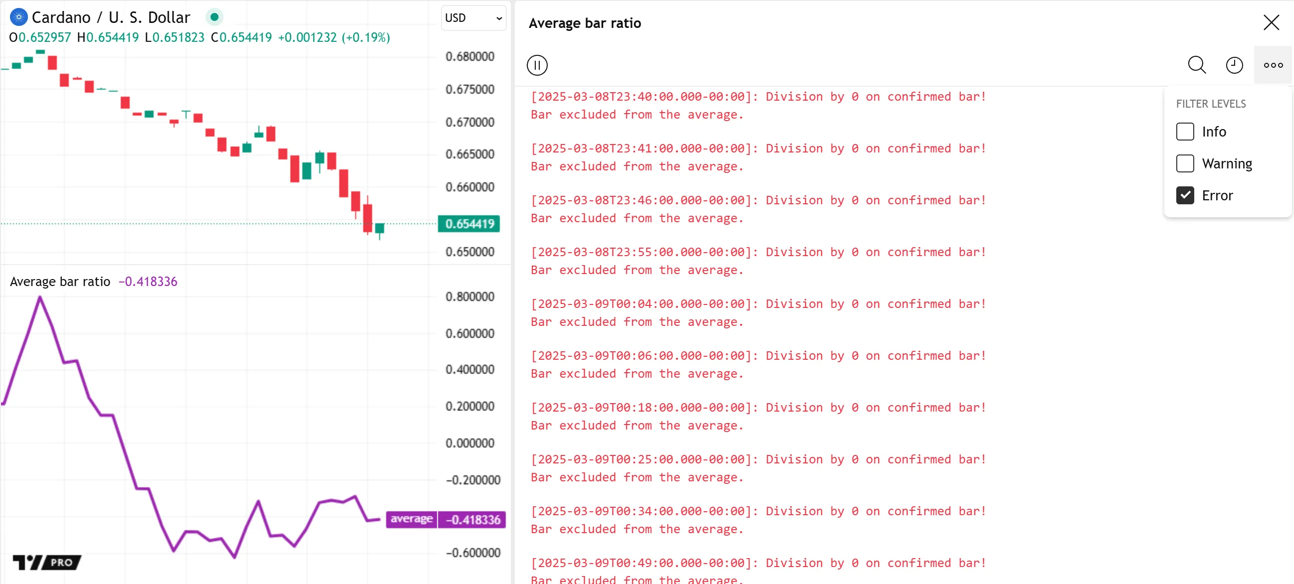
Selecting the rightmost icon above the messages in the Pine Logs pane opens a “Filter levels” dropdown menu containing checkboxes for each logging level (“Info”, “Warning”, and “Error”). To remove logs with a specific logging level from the displayed results, uncheck the level from this menu.

In the example below, we deactivated the “info” and “warning” levels for our script’s logs, allowing only “error” messages in the Pine Logs pane:

Note that:

• Deactivating logging levels in this menu hides the relevant messages but does not stop the execution of those log.*() calls in the code. For instance, a log.info() call still executes and adds to the historical log count even when the “Info” option is unchecked.

Start date

The “Start date” option above the logs in the Pine Logs pane opens a dialog box where users can specify a starting date and time to filter the displayed messages:

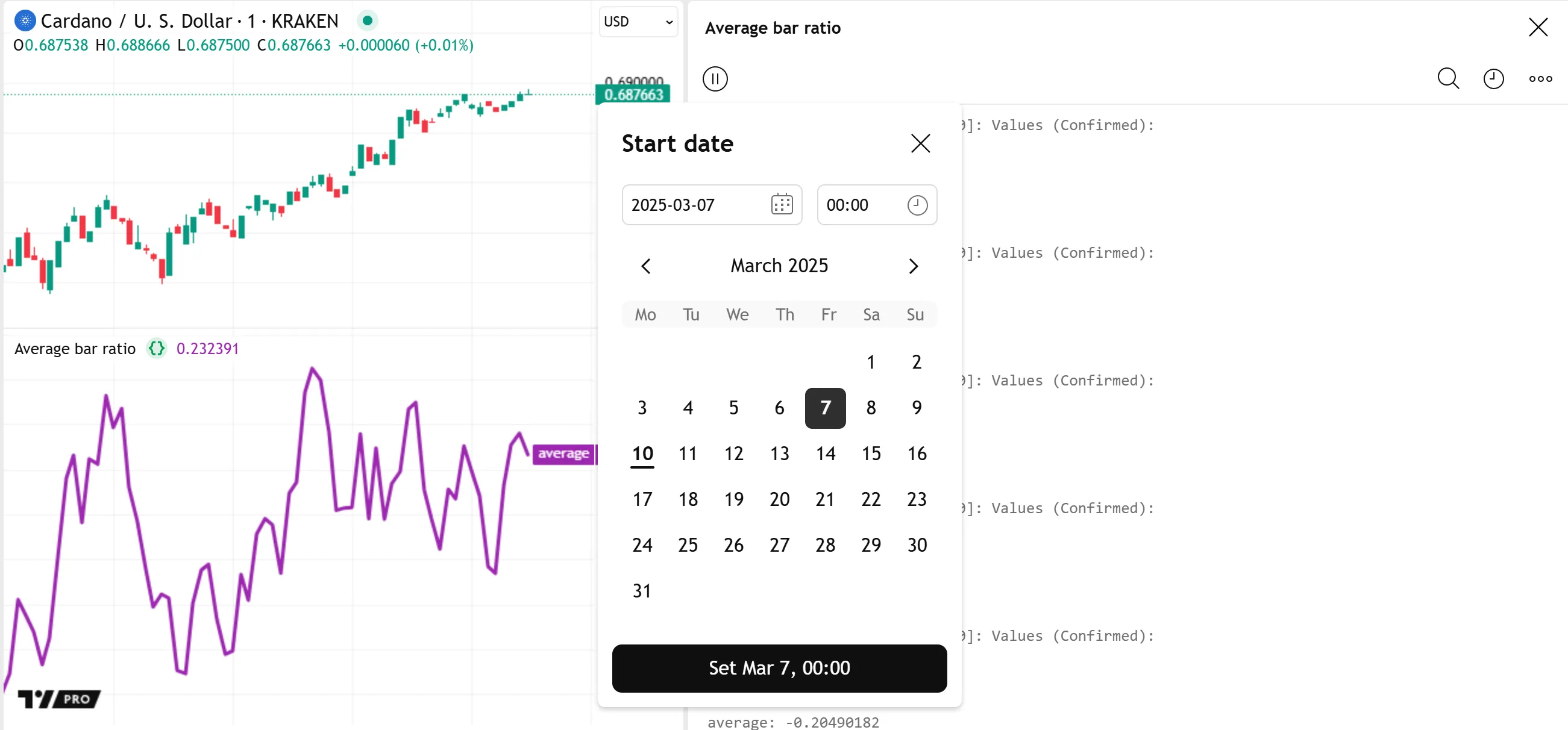
After the user sets the filter in the dialog box, a tag showing the selected date and time appears above the logs, indicating it is active. With this filter, only logs with prefixed timestamps from the specified start point onward appear in the Pine Logs pane:

Character and pattern search

The “Search” option above the logs in the Pine Logs pane opens a search bar where users can match logs containing specific character sequences or patterns, similar to the Pine Editor’s “Find/Replace” tool for matching code.

When the search bar is not empty, the pane shows only the messages that fully or partially match the text or pattern, with the matched portion of each message highlighted in blue for visual reference.

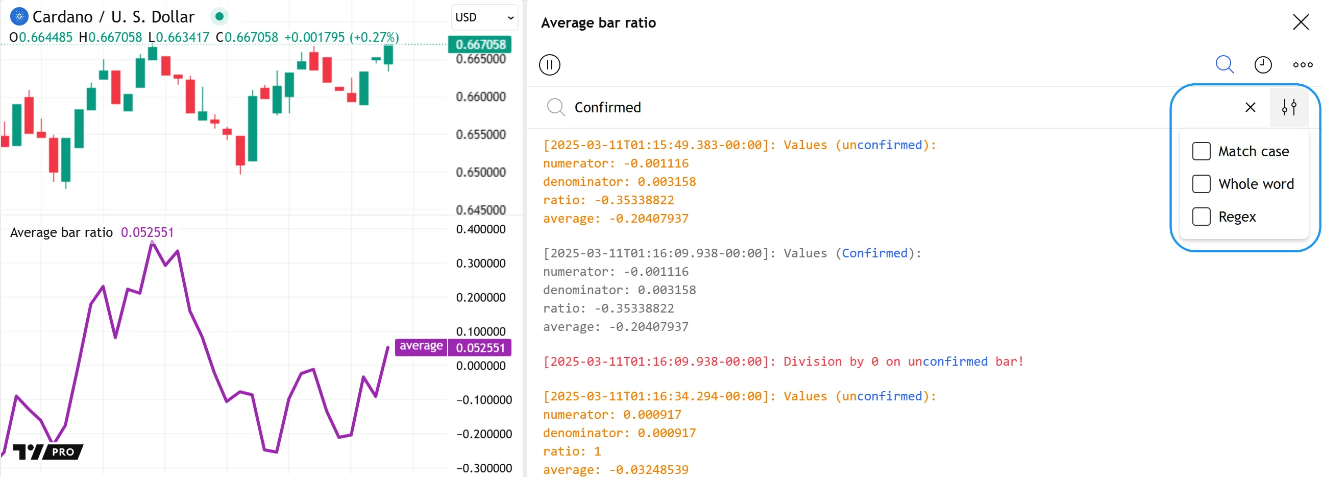
Below, we searched “Confirmed” to identify all logs from our example script that contain the term anywhere in their text:

Note that:

• The filtered results include logs containing “confirmed” with a lowercase “c” because the search filter performs case-insensitive matching on ASCII characters by default.
• The results also include logs containing “unconfirmed” because the default filter behavior does not exclusively match whole-word terms.

The rightmost icon in the search bar opens a dropdown menu containing three options to adjust the search filter’s behavior: Match case, Whole word, and Regex:

Match case

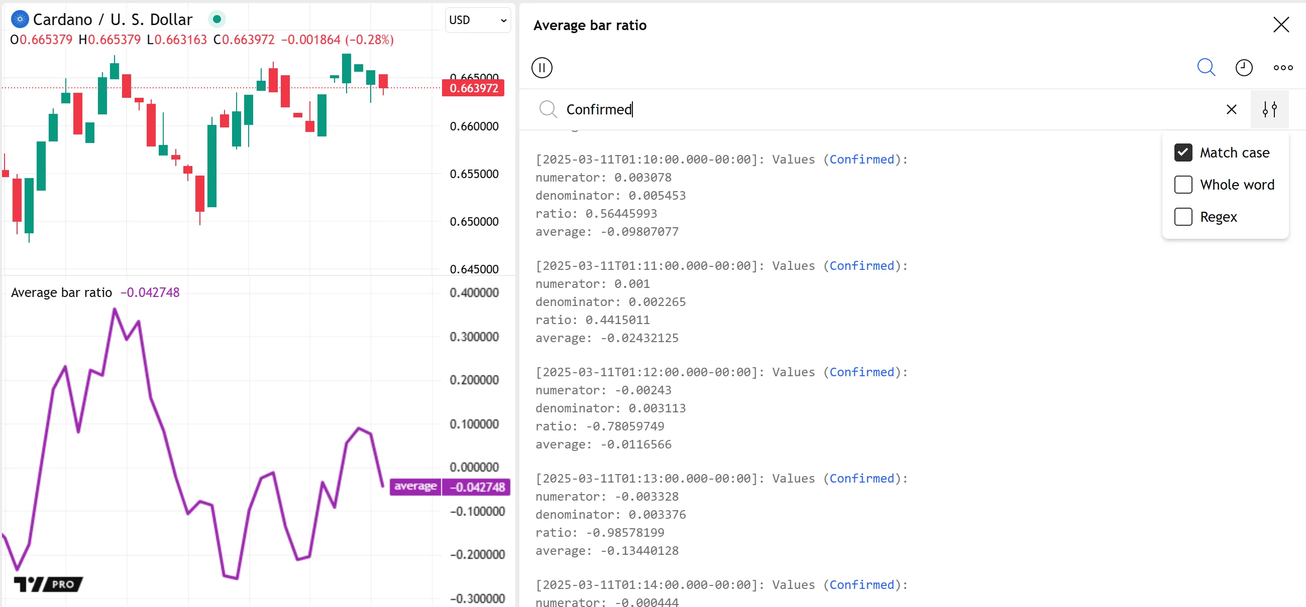
The “Match case” search option activates case-sensitive matching. With this setting, the filter’s results include only the logs containing the search query with identical cases for ASCII letter characters.

Here, we enabled the “Match case” setting for our “Confirmed” search, preventing all the script’s logs containing “confirmed” with a lowercase “c” from appearing in the results:

Note that:

• The “Match case” setting does not affect the search behavior for Unicode letter characters outside the ASCII range (U+0000 - U+007F).

Whole word

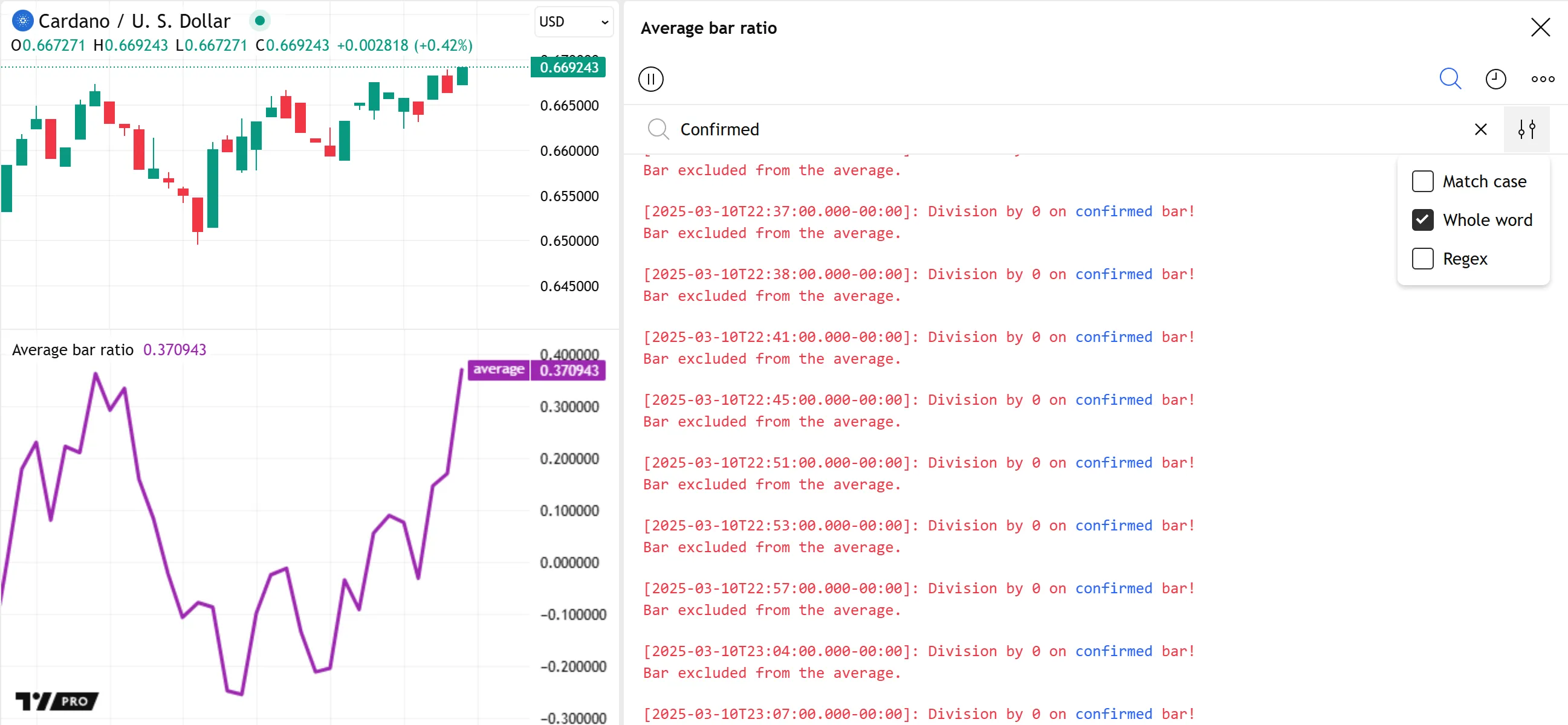
The “Whole word” search option activates whole-word matching. With this setting enabled, the filter includes logs containing the searched term, but only if it is separated from other text by whitespace characters or any of the following non-word characters: . (period), , (comma), : (colon), ; (semicolon), ' (apostrophe), or " (quotation mark).

For example, searching for “Confirmed” in our script’s logs with the “Whole word” setting prevents the messages containing “unconfirmed” from appearing in the results:

Note that:

• With the “Whole word” setting active, the search filter cannot match terms containing whitespaces or the other non-word characters listed above.
• Whole-word search queries can include other Unicode characters outside the ASCII range.

Regex

The “Regex” search option enables advanced, flexible log filtering with regular expressions (regex). In contrast to plain text searches, which only match literal character sequences, regex searches can match variable text patterns based on the rules defined by the query’s syntax.

With regular expressions, the Pine Logs search filter can isolate logs containing various text structures, simple or complex, such as dates and times with a defined format, alphanumeric sequences with varying digits or letters, sequences of characters within specified Unicode subsets, and more.

For instance, this regex search query specifies that the displayed logs must contain “average:”, with optional trailing whitespace characters, followed by a sequence of characters representing a number greater than 0.5 and less than or equal to 1.0:

average:\s*(?:0\.5\d*[1-9]\d*|0\.[6-9]\d*|(?:1\.0*|1))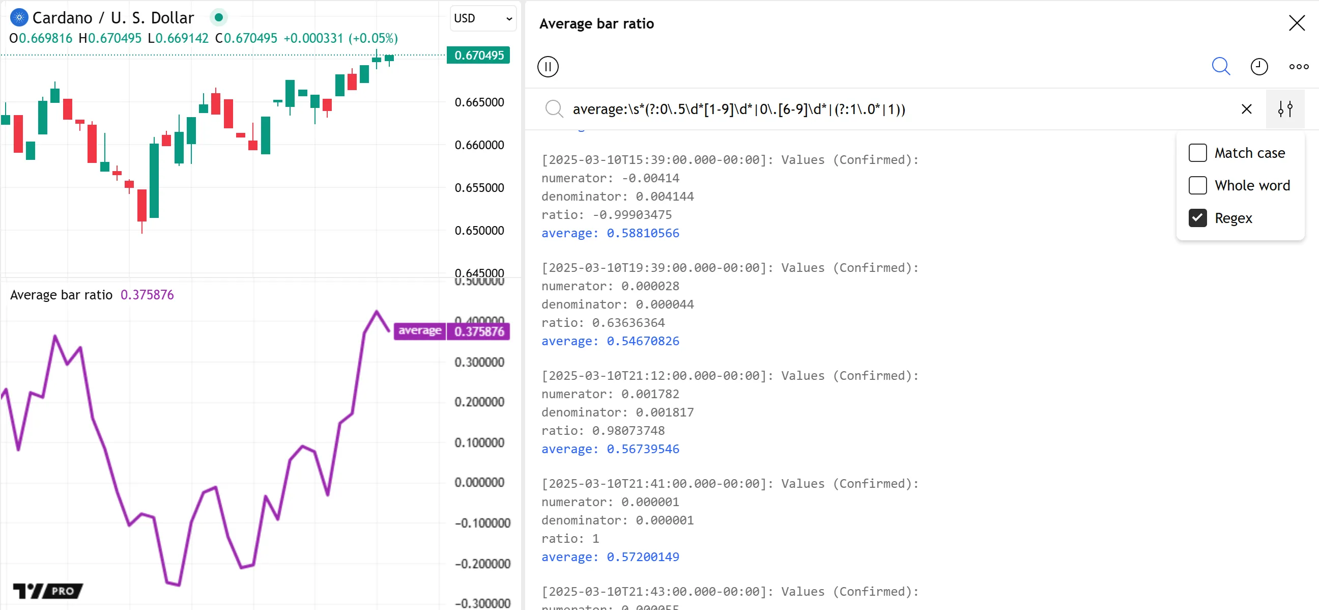

The more advanced search query below specifies that the logs must contain prefixed timestamps representing any time of day equal to or after 09:30 and before 16:00 in the chart’s time zone:

(?<=^\[\d{4}-\d{2}-\d{2}\x54)(?:09:3\d:[0-5]\d\.\d{3}|1[1-5]:(?:[0-5]\d[:\.]){2}\d{3})

For more information about regular expressions, consult the Regex syntax reference in this manual’s Strings page. Most of the described syntax works the same within the Pine Logs search filter, with a few notable differences:

• The strings used as regex arguments in str.match() calls require two consecutive backslashes (\\) for specifying escape sequences in the pattern (e.g., "\\w" means the regex matches a character from the \w class). In contrast, the Pine Logs search filter requires only a single backslash for escape sequences. Double backslashes in the search bar match the literal \ character.
• The regex search query can use the syntax \xhh or \uhhhh to reference Unicode code points in the Basic Multilingual Plane, where each h is a hexadecimal digit (e.g., \x67 and \u0067 refer to U+0067, the a character). However, the full-range syntax (\x{...}) is not supported.
• The search query cannot use Unicode property references, such as \p{Lu}, \p{IsGreek}, etc.
• The search query can use only the ^ and $ boundary assertions to match a logged message’s start and end boundaries. The \A, \Z, and \z assertions are not supported.
• The search query cannot use pattern modifiers globally (e.g., (?m)^abc). However, it can use some modifiers locally inside non-capturing groups (e.g., (?m:^abc)).

Custom code filters

If the filtering options in the Pine Logs pane are not sufficient, programmers can control specific log.*() calls using inputs and conditional logic.

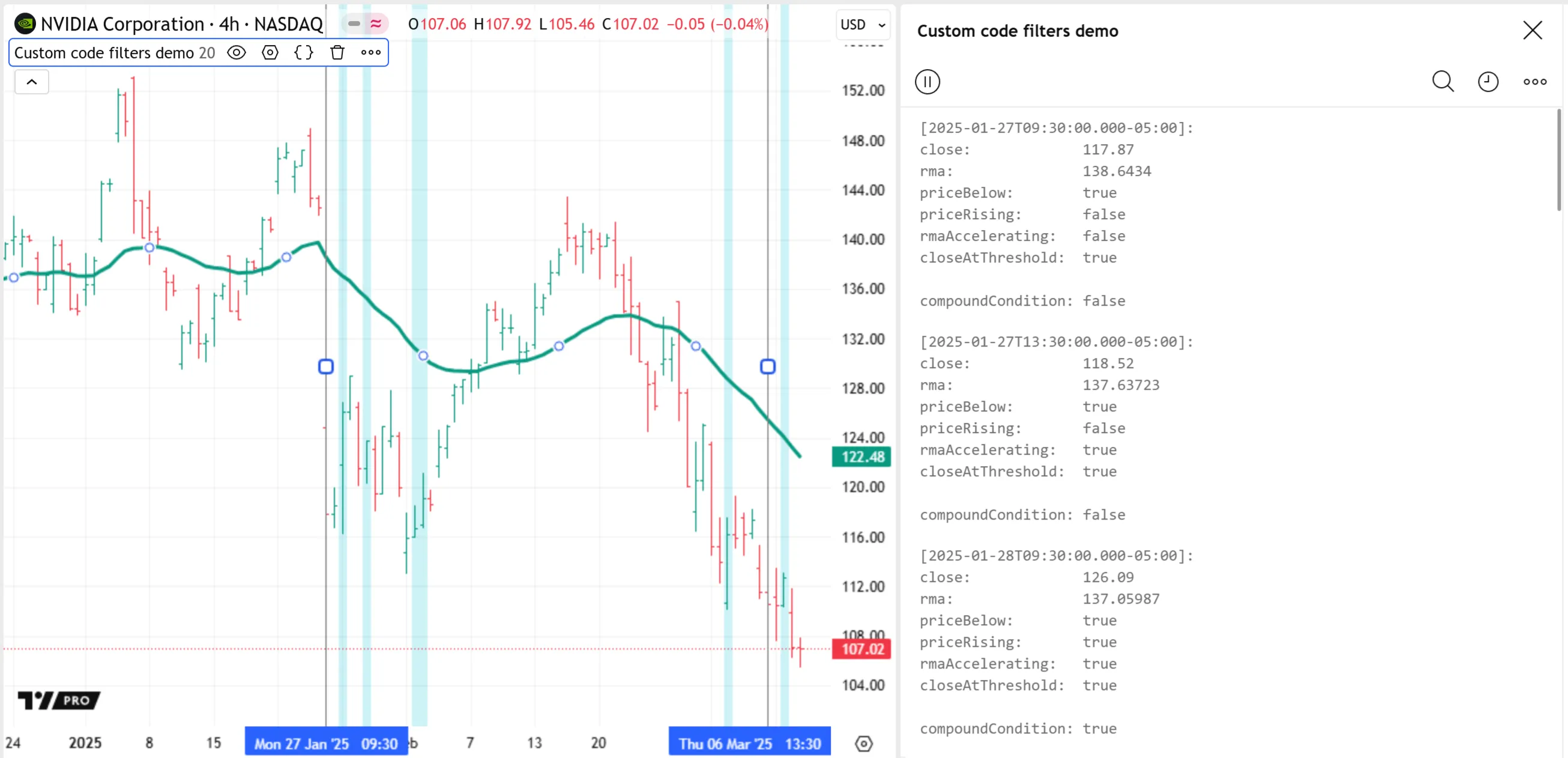
The script below calculates an RMA of close prices and creates a compound condition from four distinct individual conditions. It plots the RMA on the chart and highlights the background when the compoundCondition value is true. For debugging, the script uses log.info() to display a formatted string representing the close and rma values, the values of all the “bool” variables that form the compound condition, and the final compoundCondition value.

The filterLogsInput, logStartInput, and logEndInput variables define a custom time filter for generating logs. When filterLogsInput is true, the script uses the time inputs assigned to logStartInput and logEndInput to filter the log.info() calls, allowing a new log only when the bar’s time is within the specified range:

Note that:

• The input.*() calls assigned to the filterLogsInput, logStartInput, and logEndInput variables include a group argument to group the inputs in the “Settings/Inputs” tab.
• Users can adjust time input values directly on the chart by selecting the script’s status line and moving the displayed time markers with the mouse pointer. Additionally, users can select “Reset points” in the script’s “More” menu to clear the inputs and choose new values.
• The formatString argument of the log.info() call uses the Em Space character (U+2003) to align the represented values vertically in the logged text. In contrast to the standard space and tab characters, leading or repeated Em and En spaces are not removed from the Pine Logs pane’s displayed messages.

Pine drawings

Pine’s drawing types create chart drawings with specified properties. Scripts can place drawings at any valid chart location during code executions on any bar. Programmers can use these types in a script’s global or local scopes to visualize numeric data, conditions, colors, and strings on the chart. The flexibility of Pine drawings makes them helpful for debugging scripts when other methods do not suffice, namely when a programmer wants to inspect information graphically outside the Pine Logs pane.

However, before debugging a script using drawings, it is crucial to note the following limitations:

• The expression argument of a request.*() call cannot depend on code that creates or modifies drawings. Likewise, an indicator that specifies another context in its declaration statement cannot create drawings from anywhere in the code. To debug code that executes on requested data, use Pine Logs instead.
• In contrast to Pine Logs, drawings do not have built-in navigation features. Therefore, users must manually scroll across the chart to inspect drawings created on specific bars.
• Scripts can maintain only a limited number of objects of each drawing type. When the number of drawings exceeds the limit, Pine’s garbage collector automatically removes the oldest ones.

The sections below explain some simple debugging methods using labels and tables. These drawings, especially labels, are the most effective for on-chart debugging because they can use dynamic strings to express information from other data types as custom text.

Labels

Labels display colored shapes and text at specified chart coordinates. In contrast to the outputs of the plotshape() and plotchar() functions, labels can display text from “series string” values that change across script executions. Programmers often use labels to visualize the logic of conditional structures and show text representing information from a script’s global or local scopes.

The most common techniques for debugging with labels include:

• Drawing a label containing key information anchored to every bar that requires inspection.
• Drawing a single label containing information from specific executions at the end of the dataset or visible chart.

Drawing on successive bars

When inspecting values of varying magnitudes or different types across bars, a simple approach is to create formatted strings containing the necessary debug information and display them in labels on each bar requiring analysis.

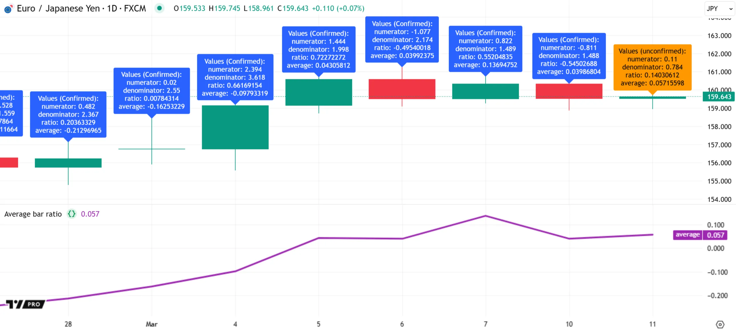
In this example, we’ve modified the “Average bar ratio” script from the Pine Logs section above. Instead of creating formatted text and displaying information using log.*() function calls, this script formats the values separately, then calls label.new() to show the results on the chart within labels anchored to each bar’s high:

Note that:

• The label.new() calls include force_overlay = true, meaning the labels always appear on the main chart pane.
• Unlike the example in the Pine Logs section, this script’s outputs are subject to rollback, meaning the information shown on a bar reflects only the bar’s latest data. The script does not show information for all realtime bar updates.

The above example allows users to inspect the script’s confirmed values or latest updates on any bar that has a label drawing. However, each bar’s results are legible only when the labels do not overlap.

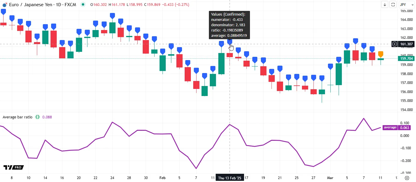
An alternative, more compact way to display text with labels on successive bars is to utilize the label.new() function’s tooltip parameter instead of the text parameter, as labels show their tooltips only when the mouse pointer hovers over them.

In the script version below, we changed all the label.new() calls to use debugText as the tooltip argument instead of the text argument. Now, we can view a specific bar’s information without visual clutter from other nearby labels:

When drawing labels across successive bars, it’s important to note that the maximum number of labels a script can display is 500. As such, the examples above allow users to inspect information for only the most recent 500 chart bars.

For successive labels on earlier bars, programmers can create conditional logic that limits the drawings to specific time ranges, e.g.:

if time >= startTime and time <= endTime
    <create_drawing_id>

Below, we added a condition to the script that draws a label only when the bar’s time is between the chart.left_visible_bar_time and chart.right_visible_bar_time values. This logic restricts the drawings to visible chart bars, allowing us to scroll through the chart and inspect labels on any bar:

Note that:

• The script restarts each time the UNIX timestamps of the chart.left_visible_bar_time or chart.right_visible_bar_time variables change after the user scrolls or zooms on the chart.

Drawing at the end of the chart

When debugging information does not change frequently across executions, or only the information from a specific execution requires inspection, programmers often display it using labels anchored to the end of the chart.

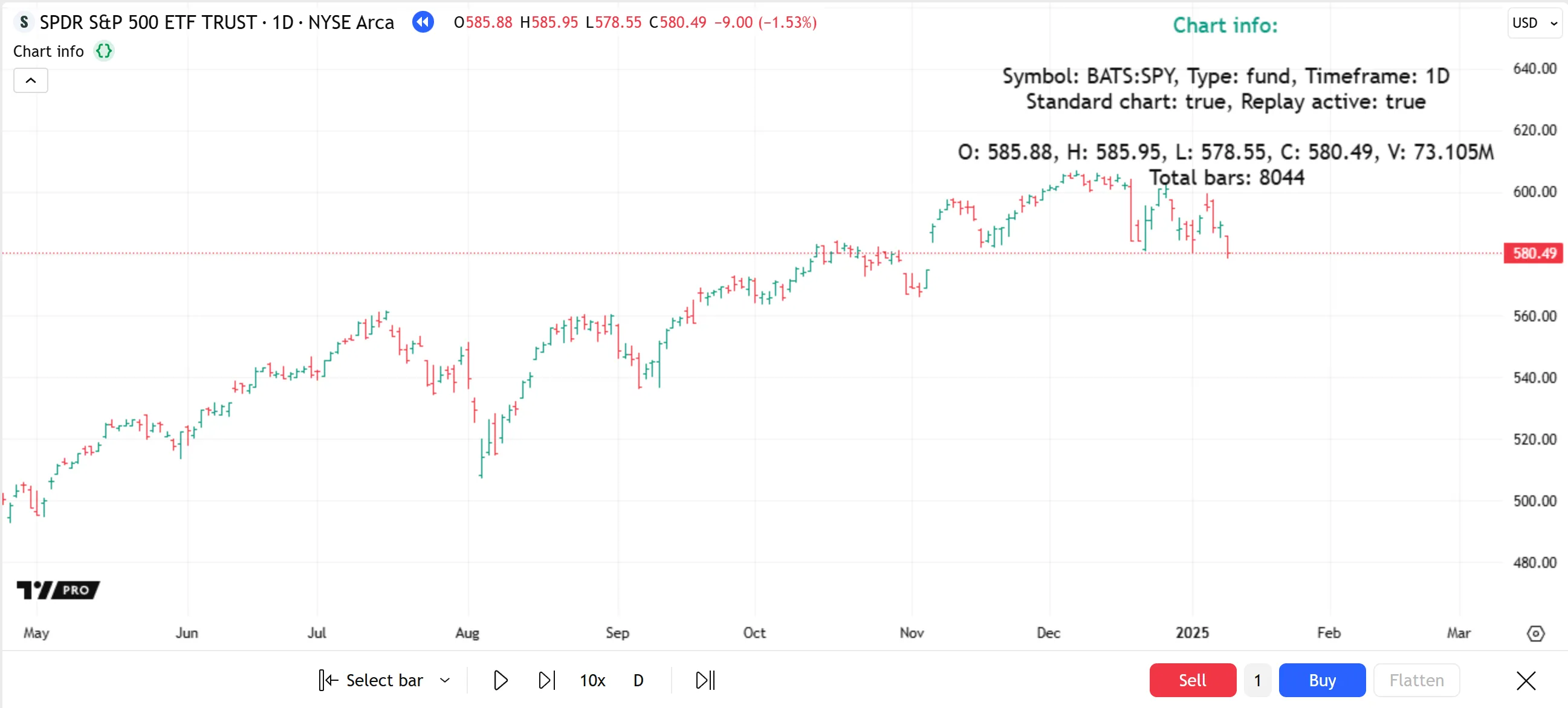
The following example displays price and chart information in four separate labels at the end of the chart. The script’s printLabel() function renders a specified string in a label that always anchors to the last available time in the dataset, regardless of when the function call occurs:

Note that:

• The printLabel() function draws one label per function call instance. The label’s x property is the maximum of the last_bar_time and chart.right_visible_bar_time values, ensuring it appears above the last available bar.
• On each execution of a printLabel() instance, the label’s text property updates to reflect the latest info value.
• The label.new() call in the printLabel() function includes force_overlay = true, meaning the drawing always appears in the main chart pane.
• This script uses four distinct printLabel() calls. The first three append repeated newline characters (\n) in the info argument to prevent the label text from overlapping.

Tables

Tables display text within cells arranged in columns and rows at fixed locations in the chart pane’s visual space. In contrast to other drawing types, which create visuals on the chart at specified coordinates, tables appear at one of nine unique, bar-agnostic locations defined by the table.position_* constants.

Because tables appear at consistent relative locations in the pane, unaffected by scroll or zoom actions, programmers occasionally use them for on-chart debugging. The most common technique is to draw a single-cell table containing information from specific script executions.

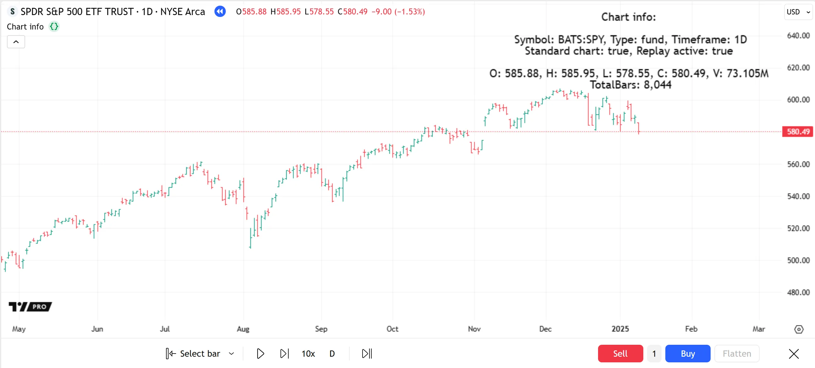
This example contains a printTable() function that calls table.new() and table.cell() to create a single-cell table that displays dynamic text in a relative location on the main chart pane. The script uses a single call to this function to display the same chart information shown by the example script from the previous section:

Note that:

• Every new table drawing replaces any existing one that has the same specified position. Therefore, scripts cannot call the printTable() function multiple times to place multiple drawings in a single location, unlike the printLabel() function from the previous section.
• This script calls printTable() only on the last historical bar and all realtime bars because updating tables on each historical bar is an unnecessary use of runtime resources. See the Reducing drawing updates section of the Profiling and optimization page for more information.

Plots and chart colors

The built-in plot*() functions display results from a value’s series in up to four locations: the chart pane, the script’s status line, the Data Window, and the price scale. Programmers often use these output functions as a quick way to display the history of a script’s numeric values, conditions, and colors. Two other functions, bgcolor() and barcolor(), color a chart pane’s background and the main chart’s bars or candles. Although not as versatile as other output functions, they offer a quick way to display conditions and colors on the chart.

All these functions, especially plot(), plotchar(), and plotshape(), can serve as helpful tools for debugging a script’s calculations and logic. For instance, the outputs of a single plot() call can show the complete available history of a script’s series on the chart and provide information for any bar in other locations.

Before using plots or chart colors for debugging, it is important to note the following limitations:

• Unlike Pine Logs or drawings, these outputs cannot display results for values that are accessible from local scopes only. Scripts must extract values from local scopes into the global scope to debug them with plots or chart colors.
• The only plot*() functions that can display text on the chart — plotchar() and plotshape() — require “const string” values. Therefore, they cannot display dynamic strings or calculated string conversions of other types.
• Similar to drawings, plots do not have built-in navigation features. Users must scroll across the chart to find plotted information for specific bars.
• The maximum plot count for any script is 64. Each call to these functions contributes a different number to the total, depending on its arguments. See the Plot limits section of the Limitations page to learn more.

Plotting numbers

One of the simplest methods to inspect global numeric series (“int” or “float” values) is to plot them using the plot(), plotchar(), or plotshape() function. The outputs on the chart pane provide a graphical view of the series’ history. The other possible output locations (status line, price scale, and Data Window) show formatted numbers representing the values calculated on a specific bar.

Let’s look at a simple debugging example. The following script calculates a custom oscillator whose value is the average of three separate oscillators. It displays the oscillator value in four output locations using a plot() call:

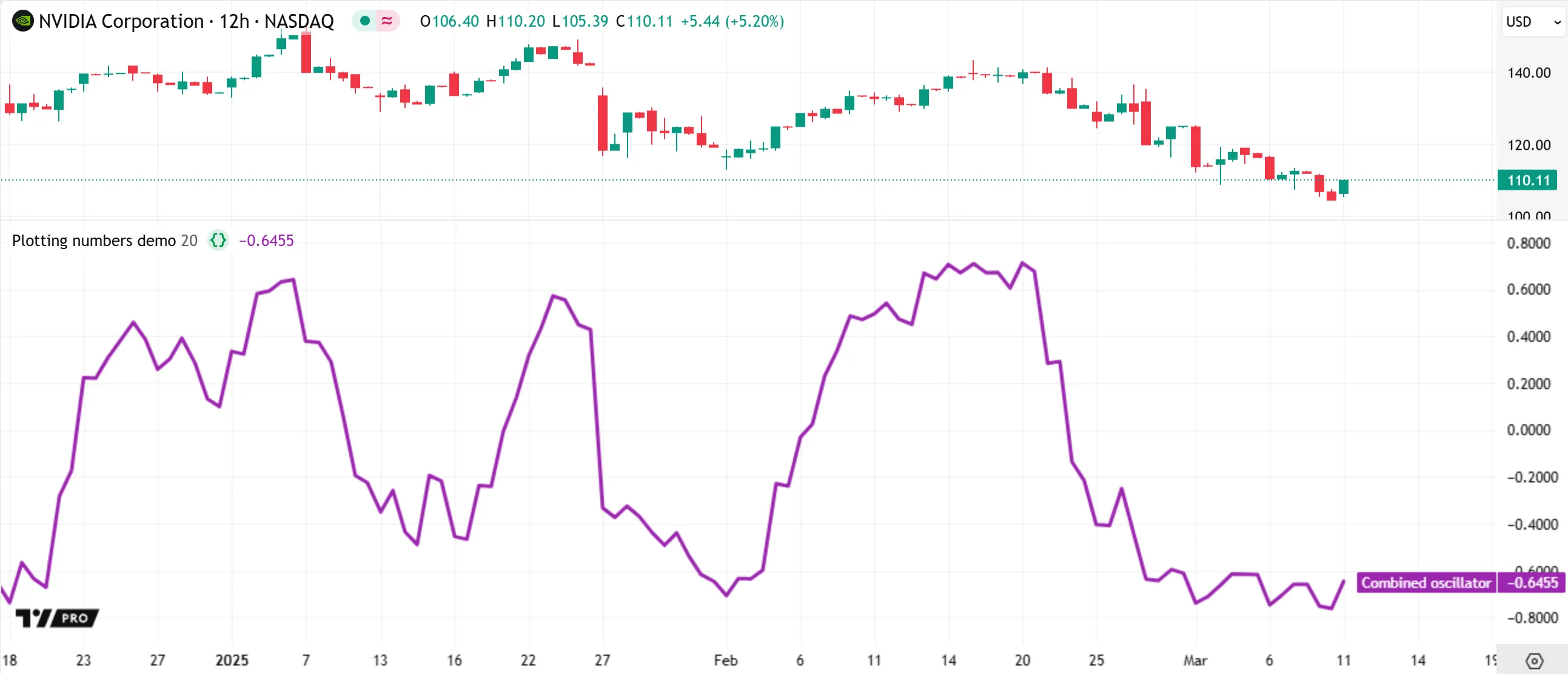
The above script’s outputs allow inspection of the final oscillator, but not the three constituent oscillators that determine its value. Because the script calculates all three series in the global scope, we can inspect them using additional plots. Here, we add three plot() calls to the script to display each oscillator, allowing us to verify the script’s calculated values and understand how they affect the final result:

Note that:

• The numbers in the script’s status line and the Data Window represent the values plotted on the bar at the mouse pointer’s location. When the pointer is not on the chart, these numbers represent the latest bar’s data.
• The labels in the price scale show the latest non-na values available in the plotted series up to the last visible bar. If a plotted series does not have a non-na value at any point before that bar, the price scale does not show a label for it.

Plotting without affecting the scale

Debugging multiple numeric series by plotting them on the chart can make the results hard to read if the plots affect the price scale, especially if each plotted series has a significantly different value range. Programmers can specify a plot’s display locations to avoid distorting the scale by passing a display.* constant or expression to the display parameter of the plot*() call.

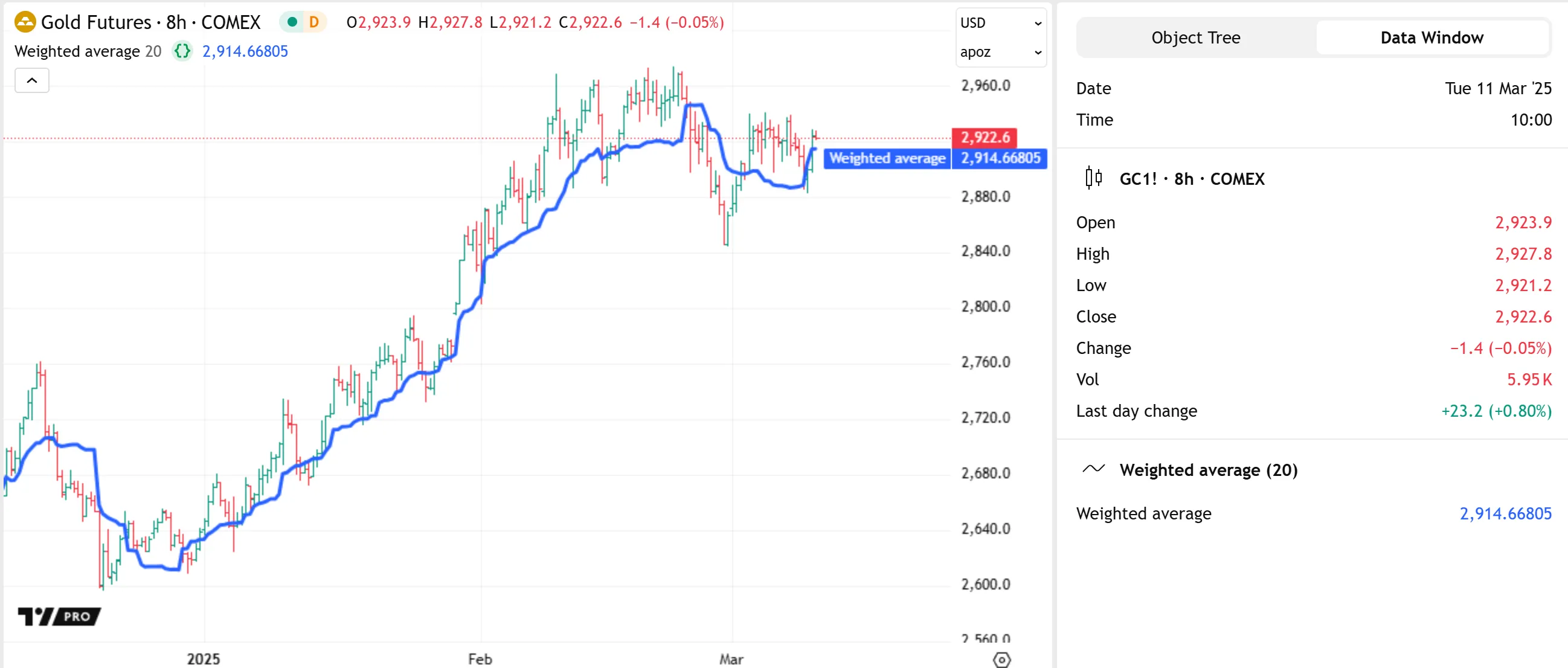
Let’s look at a simple example that calculates a few numeric series with different ranges. This script calculates a weighted moving average with custom weights and plots the result on the chart:

Note that:

• This script includes precision = 5 in the indicator() declaration statement, which specifies that it plots numbers with five fractional digits instead of using the chart’s default precision setting.

Suppose we want to inspect all the values in the average calculation using plots. If we use plot*() functions with the default display argument (display.all), the plotted results appear in all possible locations, including the chart pane. Unlike the example script from the Plotting numbers section, this script’s visuals become hard to read in the pane because each plot has a significantly different range:

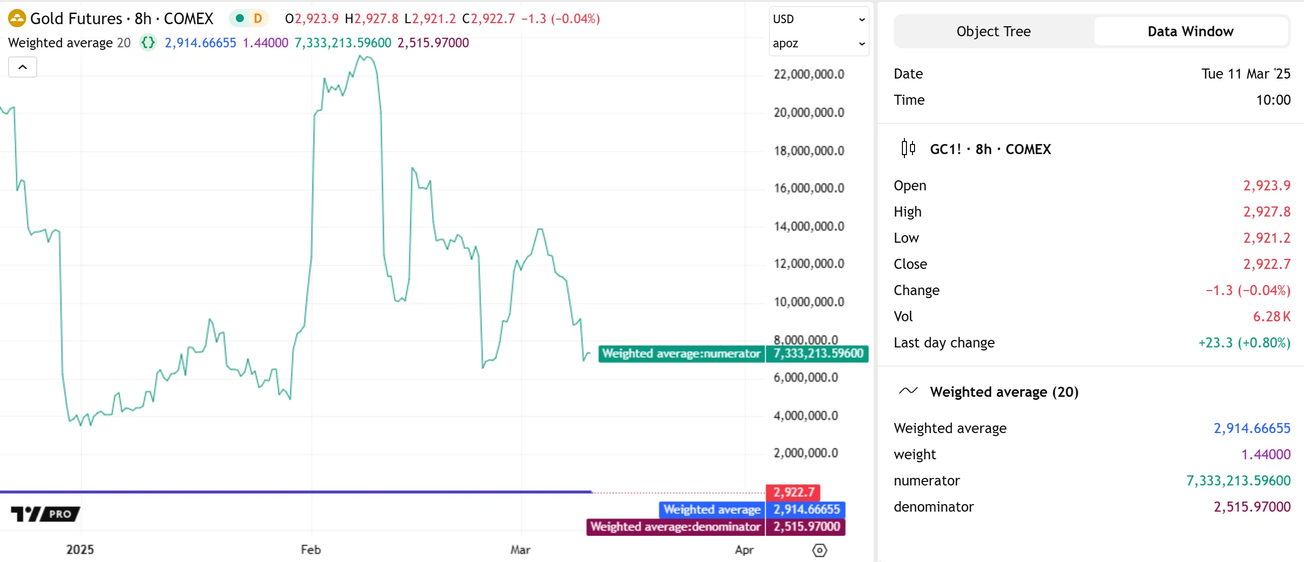
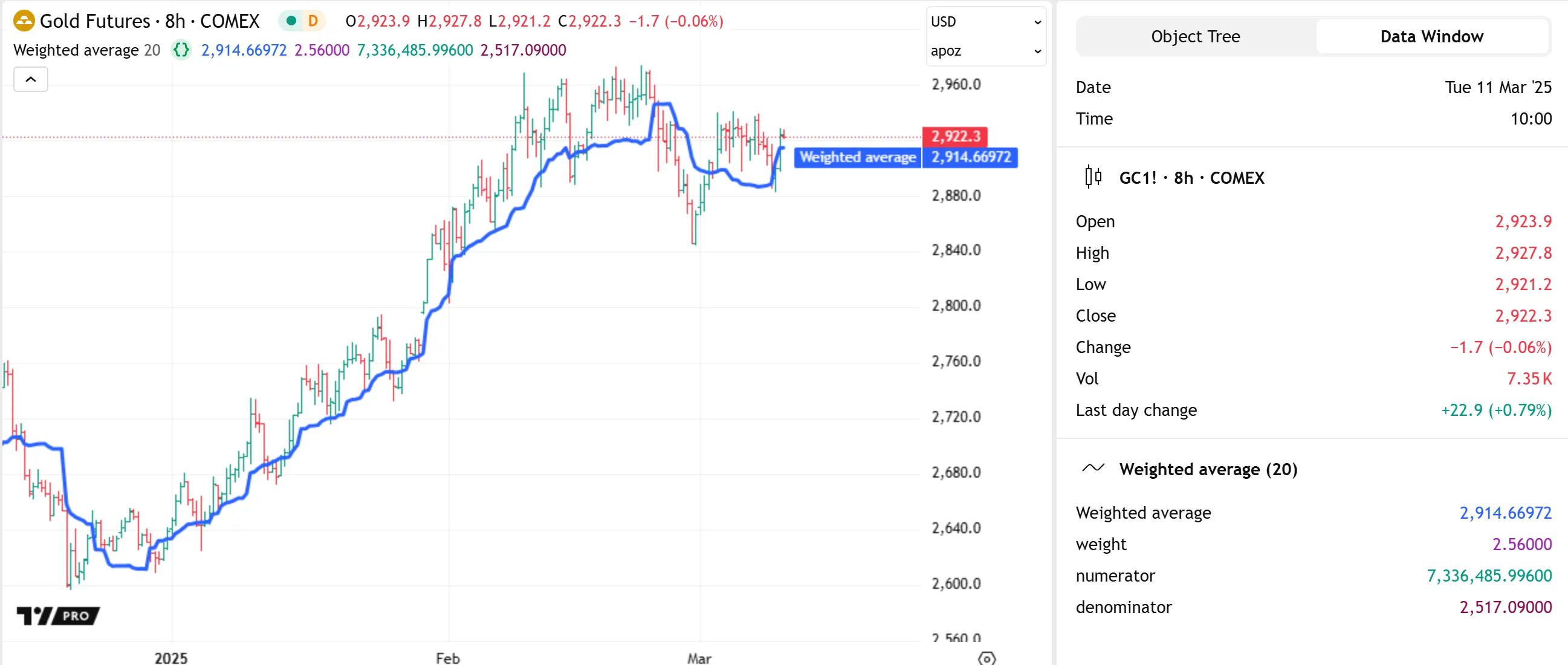
We can change the display argument in each debug plot() call to view all the calculated values while preserving the chart’s scale. Below, we set the argument to display.all - display.pane, meaning all the debug plots show information in all locations except the chart pane. Now, we can visualize how the calculated values affect each bar’s average result without distorting the scale:

Note that:

• The display.* constants support addition and subtraction operations for customized display settings. This script uses subtraction to remove display.pane from the output locations allowed by display.all. Operations that remove valid display constants more than once do not cause errors. For instance, this script produces the same outputs if it subtracts display.pane once, twice, or more times in the debugLocations expression.

Plotting and coloring conditions

Programmers can inspect a script’s conditions (“bool” values) with the plot*(), bgcolor(), and barcolor() functions in several ways, including:

• Using the “bool” condition as the series argument in a plotshape() or plotchar() call. The call creates a shape/character with specified text on the chart when the condition is true, and it shows a numeric text representation of the condition in the status line and Data Window (1 for true and 0 for false).
• Creating a logical expression that returns different “int” or “float” values for the condition’s true and false states, then using the result as the series argument in a plot*() call. When using plotchar() or plotshape(), note that these functions show visuals on the chart only when the series value is not na or 0.
• Creating a logical expression that returns different “color” values based on the condition’s true or false state, then using the result to color the chart with bgcolor() or barcolor(), or to color a plot or fill.

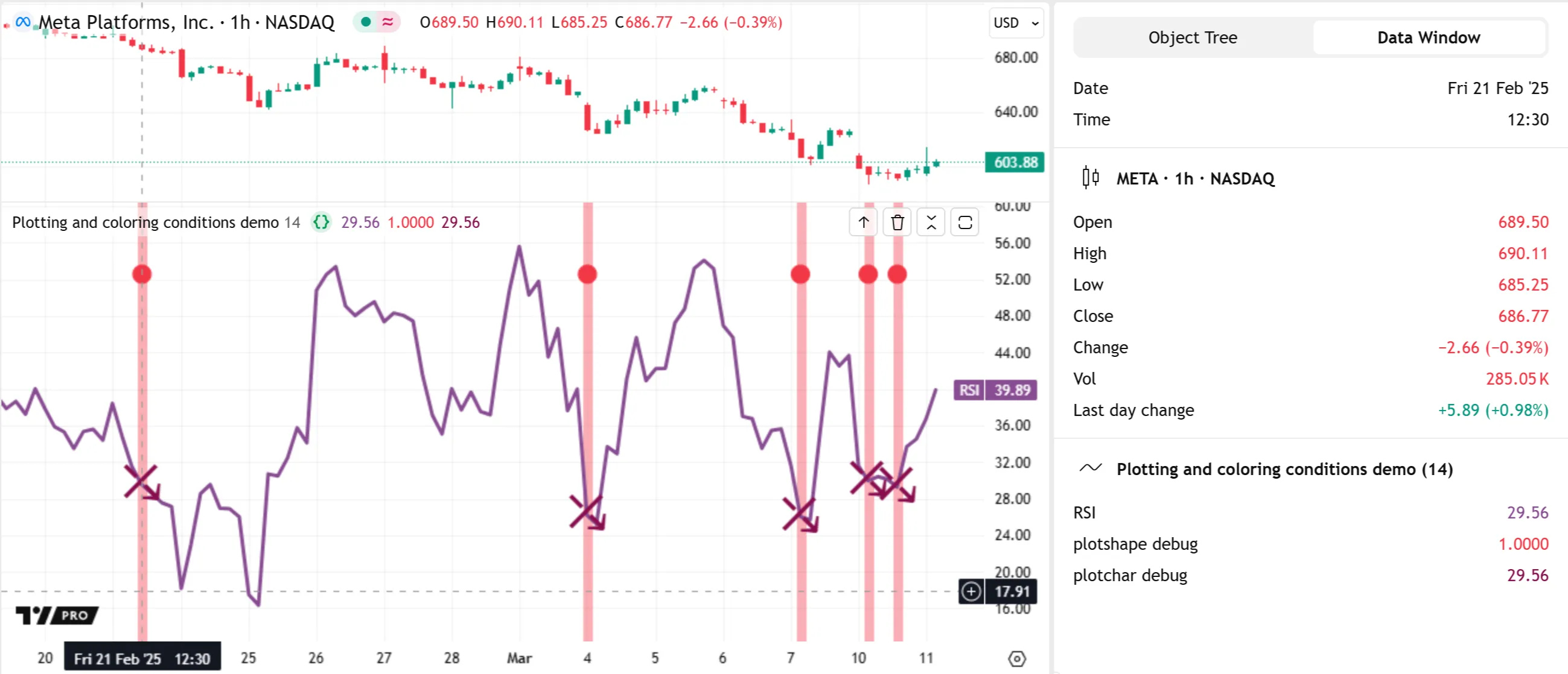
The following example uses the above methods to debug a simple condition. The script calculates an RSI with an input length and defines a crossBelow condition that is true when the RSI crosses 30. It uses plotshape(), plotchar(), and bgcolor() calls to visualize the crossBelow condition in different ways:

Note that:

• The plot*() functions that display text or shapes on the chart — plotshape(), plotchar(), and plotarrow() — do not display data in the price scale.
• The plotshape() call uses crossUnder as its series argument. The chart pane shows a shape at the top when the condition occurs. The status line and Data Window show 1 when the series is true and 0 when it is false.
• The plotchar() call plots the result of a ternary expression that returns the rsi when crossUnder is true and na otherwise. It shows the character U+2930 at the rsi location when the expression does not evaluate to na. Because the series argument is a “float” value, the number in the status line and Data Window represents that value directly.
• The bgcolor() call highlights the chart’s background when crossUnder is true, but it does not display information in the status line or Data Window.

The plotshape() and plotchar() functions have a text parameter that adds “const string” text to the plotted shapes/characters. When debugging multiple global conditions, it is often helpful to call these functions with text arguments to label each condition for simple on-chart inspection. The arguments can contain the newline character (\n escape sequence), allowing scripts to plot multiple shapes in identical locations with non-overlapping text.

Let’s explore a debugging example using this approach. The script below calculates an RSI and its median over lengthInput bars. Then, it creates five singular conditions and uses them to form a compound condition. The script plots the rsi and median values with the plot() function, and it colors the background with bgcolor() when the compoundCondition is true:

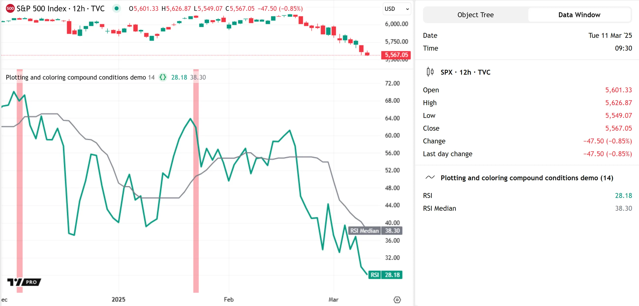
To verify that the script’s logic works as intended, we can inspect each of the conditions that affect the final compoundCondition value. Below, we added five plotchar() calls to display information for these conditions, each with the same location argument. To label the conditions on the chart, each plotchar() call uses a string containing newline characters (\n) and a digit from 1 to 5 as the text argument. With these outputs, we can see which sets of conditions trigger each compoundCondition occurrence:

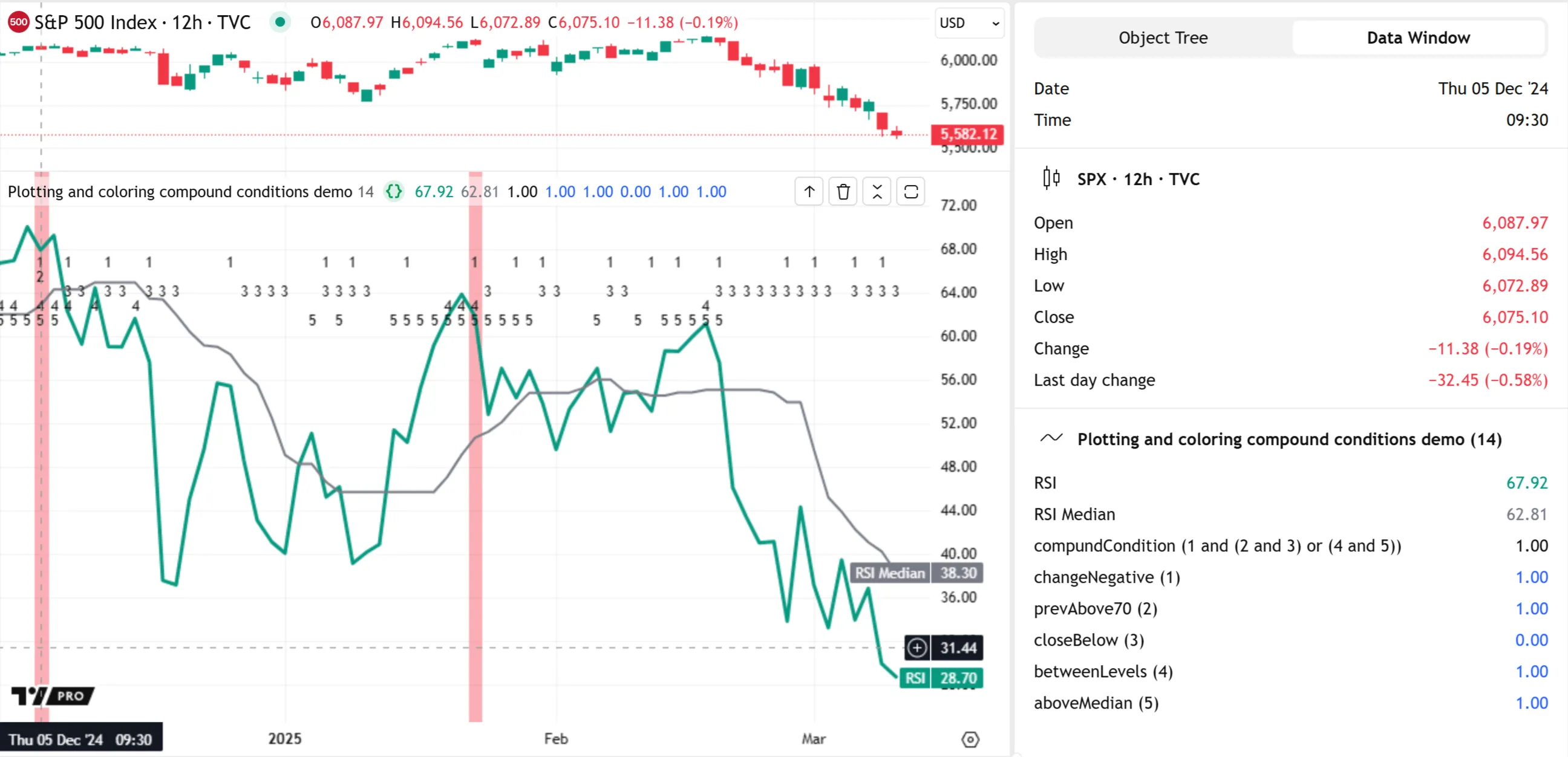
Note that:

• The char argument of each plotchar() call is an empty string, meaning the function displays its text value without a character above it.
• Because each plotchar() call outputs results at the same relative location (location.top), we included different numbers of leading \n sequences in the text arguments to move the displayed numerals down and ensure they do not overlap.
• The title argument of each plotchar() call contains the condition number to distinguish it in the Data Window.
• The plotshape() call’s title describes the compound condition’s structure in the Data Window.

To learn more about the plotshape() and plotchar() functions and how their outputs differ from labels, refer to the Text and shapes page.

Tips and techniques

The following sections explain several additional tips and helpful techniques for effective Pine Script debugging.

Decomposing expressions

One of the best practices for efficient debugging is to split expressions, especially those with multiple calculations or logical operations, into smaller parts assigned to separate variables. Decomposing expressions enables programmers to inspect each critical part individually, making it easier to verify calculations or logic and isolate potential issues in the code. Additionally, complex code broken down into smaller parts is typically simpler to read, maintain, and profile.

The following script calculates a custom oscillator representing the smoothed median change in the differences between the close price and two EMAs over different lengths. The script performs all the calculations in a single expression assigned to the osc variable. Then, it creates a compound condition in another expression assigned to the upSignal variable and uses that variable to trigger order placement commands. The script plots the osc series as columns with different colors based on the upSignal value:

Because the osc and upSignal values depend on multiple calculations and conditions, inspecting only the final values does not provide complete information about the script’s behaviors. To verify the script’s workings, we can decompose the expressions assigned to osc and upCondition into smaller parts and inspect them individually.

The script version below declares several extra variables to hold different parts of the original osc and upCondition expressions. With this expanded structure, we can inspect each part of the calculations and logic step-by-step using various outputs. In this script, we included a single log.info() call at the end that displays formatted text containing each variable’s information in the Pine Logs pane:

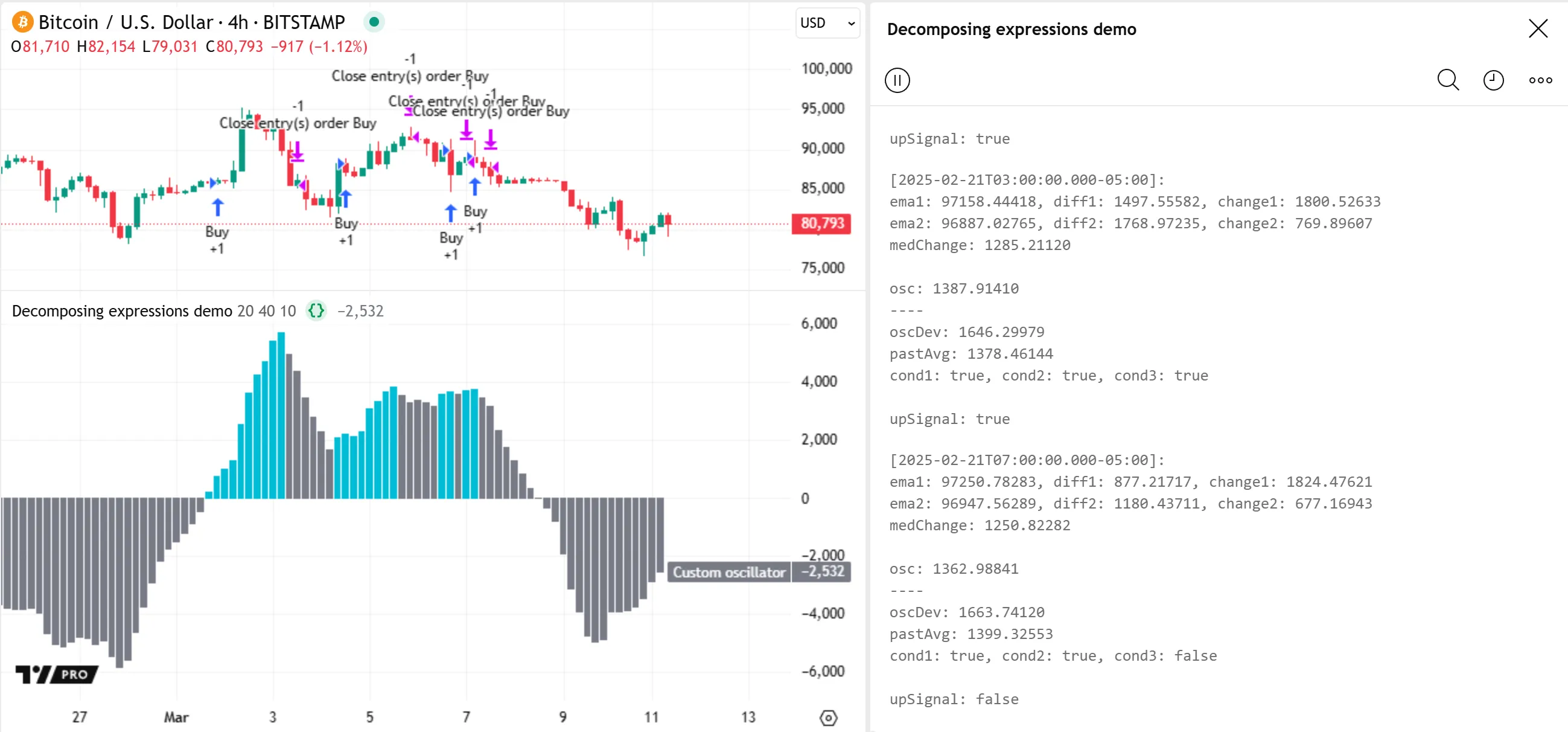
Note that:

• This script declares some extra variables on the same line, separated by commas, to reduce the number of lines added to the code.
• The script calls log.info() only when barstate.isconfirmed is true, preventing unnecessary logs on the ticks of unconfirmed bars.
• All the placeholders with the number modifier in the log.info() call’s formatting string include the 0.00000 pattern, which forces the formatted numbers to always show five fractional digits. Refer to the Formatting strings section of the Strings page for more information.
• The Pine Logs pane displays up to 10,000 historical logs. To view earlier logs, add another condition to the if structure that limits the log.info() call to specific bars. See the Custom code filters section above for an example that restricts log.*() calls using time inputs.

Extracting data from local scopes

The scope of an identifier (e.g., a variable) refers to the part of a script where it is defined and accessible during the script’s execution.

All identifiers declared outside user-defined functions, methods, loops, conditional structures, or user-defined type and enum type declarations belong to the global scope. Identifiers in the global scope are accessible to most inner (local) scopes after declaration. Every Pine script has exactly one global scope.

All user-defined functions, methods, loops, and conditional structures in a script create unique, separate local scopes. All identifiers within a local scope belong exclusively to that scope, meaning their values or references are inaccessible to any outer or containing scope.

A common practice when debugging variables declared in a local scope is to extract their data to an outer scope or the global scope, making it usable in debugging outputs with different scope requirements.

The following sections explain techniques for extracting data from local scopes using return expressions and reference types. We demonstrate these techniques on the following script, which contains a customMA() function that calculates a custom adaptive moving average of a source series based on the distance from its current value to its 25th and 75th percentiles over length bars. The script contains a local function scope, and a nested block scope from the if structure that sets the outerRange value:

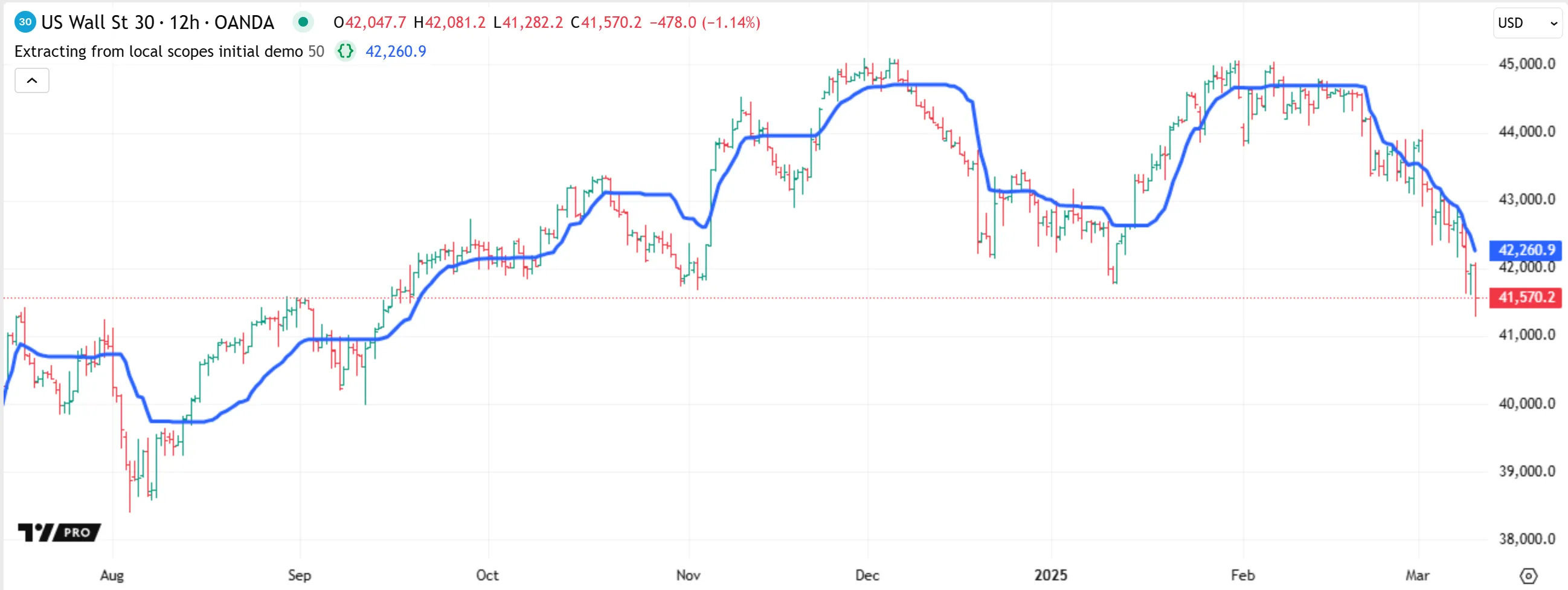
Extraction using return expressions

In Pine Script, any user-defined function or method call, loop, or conditional structure returns the result of the final expression or nested structure within its local scope. Scripts can use these structures’ returned results, excluding void, by assigning them to variables declared in the outer scope.

When debugging functions and conditional structures that contain multiple local variables, a common technique to extract data from their scopes is to return tuples containing the data that requires inspection.

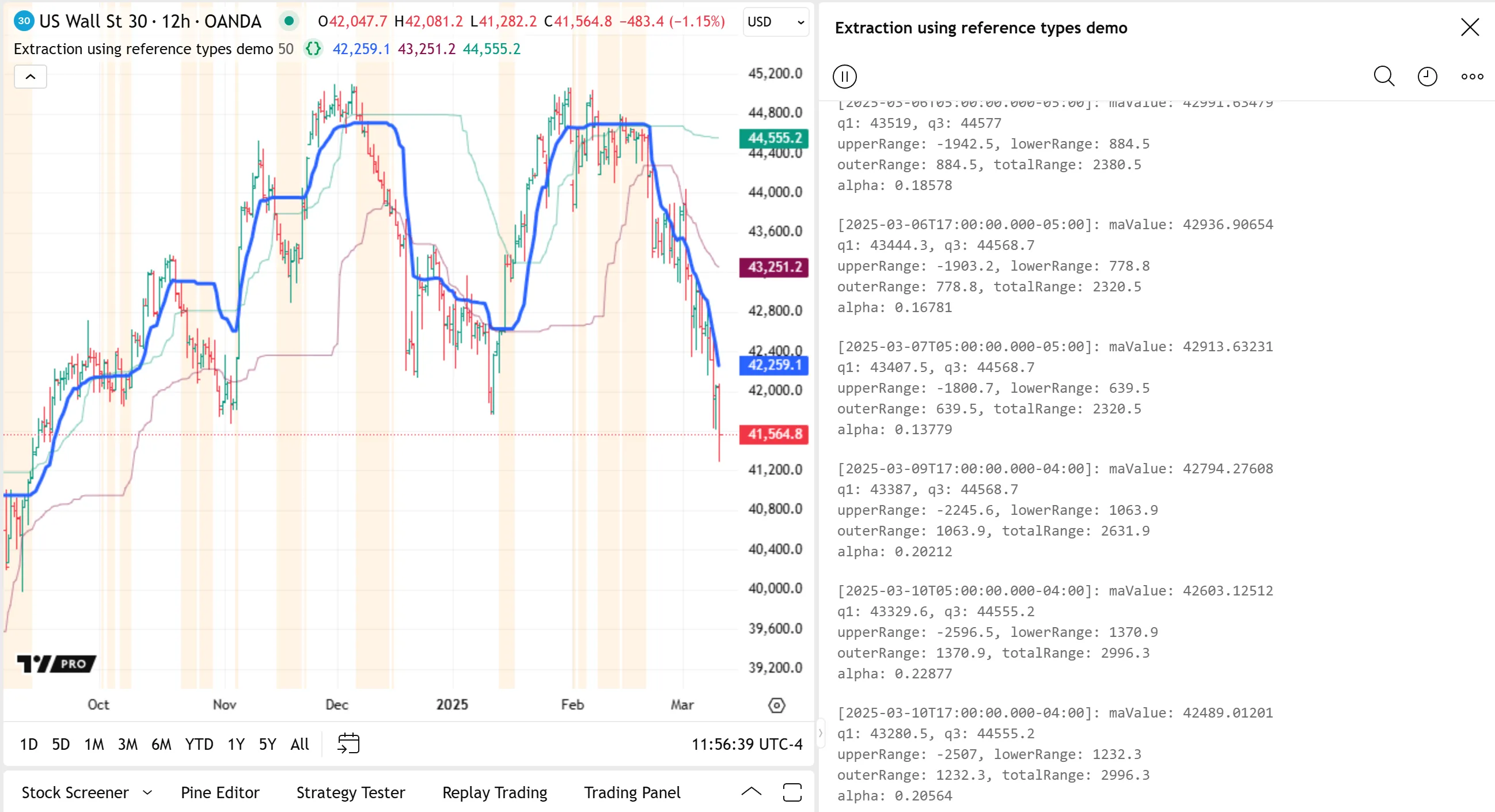
Here, we’ve modified the previous example script’s customMA() function to return a tuple containing values calculated from the local scopes. With this change, the script can call the function with a tuple declaration to make all the data available to the global scope. The script plots the q1Dbg and q3Dbg values, highlights the background when alphaDbg is 0, and uses log.info() to display a formatted string containing all the extracted data in the Pine Logs pane:

Note that:

• We added a tuple at the end of the if structure’s block to return the upperRange and lowerRange values from its local scope. The function assigns the result to a two-variable tuple in its main scope, enabling it to include the if structure’s local values in the return expression.

Extraction using reference types

Reference types, including all special types and user-defined types (UDTs), serve as structures for creating objects. Each object has an associated reference that distinguishes it and provides access to its data. Unlike fundamental types, variables of reference types do not store values directly. Instead, they hold the references for specific objects in memory.

An advanced, flexible way to extract data from local scopes is to initialize reference-type objects — such as instances of collections or UDTs — in the global scope and store local variable data in their elements or fields.

This technique is especially useful for extracting data from user-defined functions and methods. Although functions can access global variables, they cannot reassign them like global conditional structures and loops can. Consequently, they cannot update the data held by global variables of fundamental types. However, scripts do not modify reference types by reassigning their variables; they access objects via their references and use methods or field reassignments to update their data. As such, scripts can update global collections or UDT instances from inside function scopes.

For example, this modified version of our initial script declares a global debugData variable that holds the reference of a map with “string” keys and “float” values. Each map.put() call inside the customMA() scope modifies the map by adding a key-value pair containing a local variable’s name and value. After calling customMA(), the script uses map.get() calls on debugData to retrieve the stored information for its debugging outputs:

Note that:

• The script declares debugData with the var keyword, meaning the assigned map reference persists across script executions.
• A function executes its local code only when the script calls it. Therefore, the debugData map contains new information only after the customMA() call.
• Because the map.put() calls in customMA() assign keys to the map that do not change across executions, each customMA() call replaces the debugData map’s existing data. Programmers can preserve data from specific executions with this technique by making a copy of the global collection after the function call.

Inspecting loops

Loops are structures that execute a local code block repeatedly based on a counter (for), the contents of a collection (for…in), or a condition (while). These structures allow scripts to perform repetitive tasks without redundant lines of code.

Because loops can execute their local code multiple times, programmers must use techniques to track local variables across iterations to debug them effectively. As with other structures, there are many ways to inspect loops. These sections cover two helpful techniques: collecting loop information and tracing loop executions.

Collecting loop information

One of the most effective loop inspection techniques is to use collections or strings to gather information from the local scope on each iteration requiring inspection, then use the information in output functions after the loop terminates.

Let’s look at a simple loop debugging example using this technique. The following script calculates the average rate of change in the close price over lengths from 1 to lookbackInput bars inside a for loop. It declares an aroc variable in the global scope, sums the rates of change inside the loop, and then divides the sum by the lookbackInput to calculate the average:

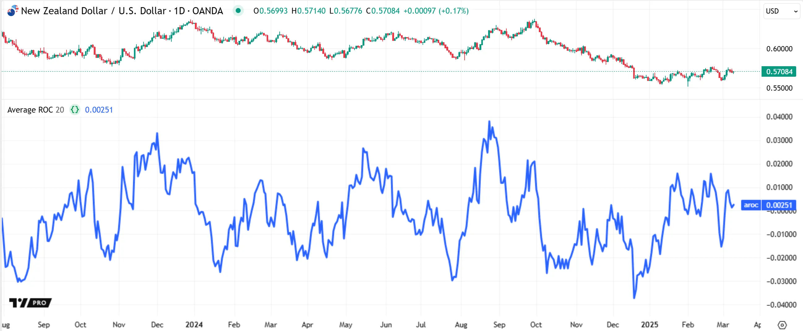
To debug the script’s loop and ensure it works as intended, we can collect data from the local scope on each iteration and pass the result to the available output functions after the loop ends. In the script version below, we demonstrate two extraction methods. The first declares a global logText variable and concatenates formatted strings containing each loop iteration’s length and roc values. The second declares a global rocArray variable and pushes each iteration’s roc value into the referenced array.

After terminating the loop, the script calls log.info() to display the logText in the Pine Logs pane if the bar is confirmed. It then displays a “string” representation of the rocArray inside label tooltips. Lastly, it shows the array’s first and last element values in all possible plot locations with the plot() function:

Note that:

• Scripts can generate Pine Logs and drawings directly from within a loop’s local scope. However, because loops usually execute their local code more than once, calling log.*() or label.new() functions inside the scope can result in numerous logs or labels per bar. Logging on each iteration helps trace execution patterns, but it also limits the number of historical bars with available debug data. See the next section, Tracing loop executions, for an example.
• Strings can contain up to 4096 characters, and large strings or repeated concatenation can impact a script’s performance. Therefore, extracting loop information with string concatenation is suitable for relatively small loops or inspecting specific variables. To extract large amounts of data from loops, use collections instead.

Tracing loop executions

An alternative way to inspect a loop, without collecting information for use in the outer scope, is to add log.*() calls directly to the loop’s local block. Each iteration that activates the call results in a new message in the Pine Logs pane, allowing programmers to trace the loop’s execution pattern in detail.

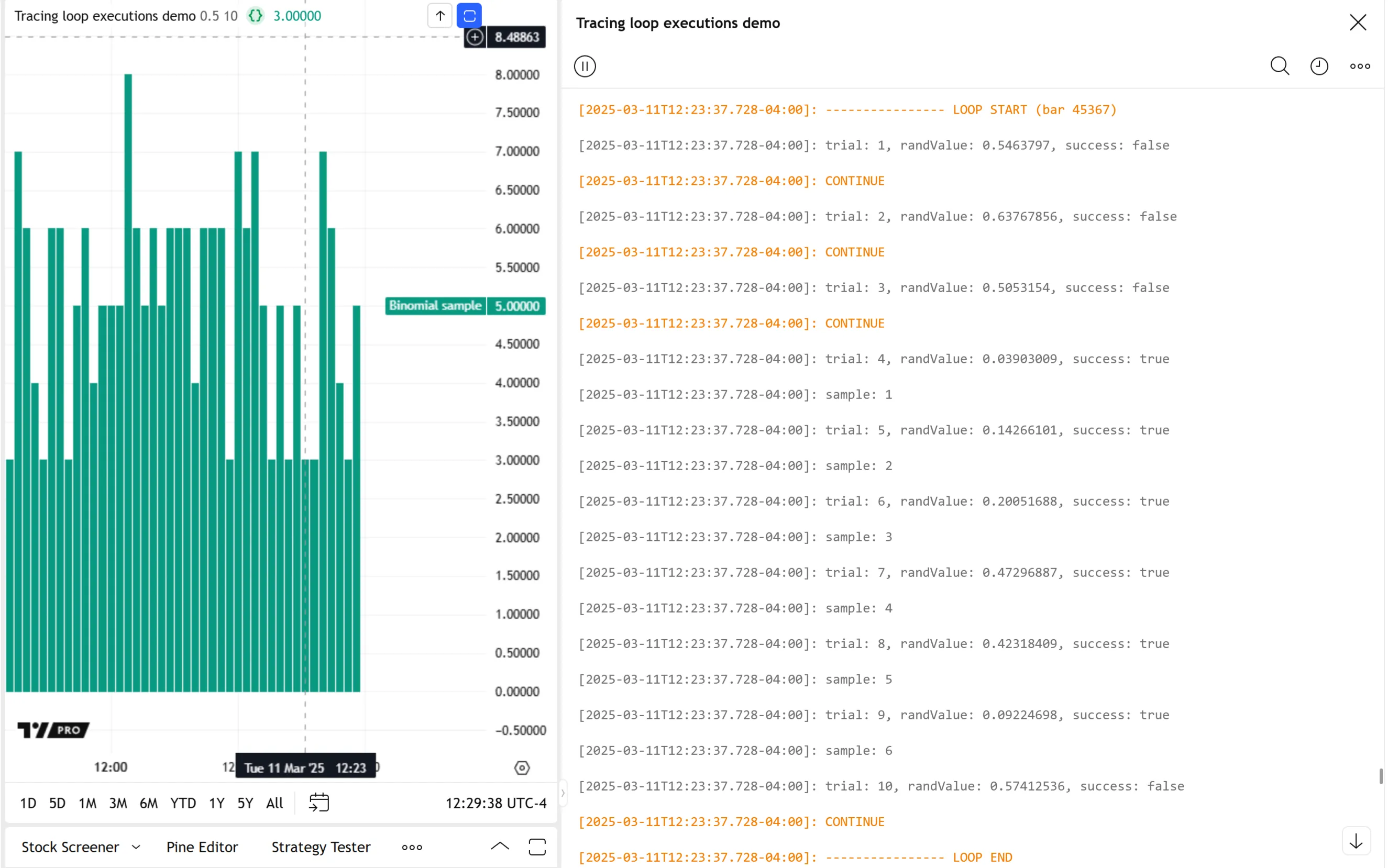
This simple script calculates a random sample from a binomial distribution using a for loop. The plotted sample series represents the number of math.random() calls across trialsInput iterations that return a value not exceeding the probabilityInput value. On each iteration where success is false, the loop skips the rest of its block and moves to the next iteration. On other iterations, it increments the sample value by one:

Below, we added log.*() function calls to generate Pine Logs at specific points in the loop’s local block across iterations. Each loop iteration creates two new logs. The first log shows formatted text containing the local trial, randValue, and success variables’ values. The second log depends on the if statement. When the statement’s local code executes, the log is a "CONTINUE" message with the “warning” level. Otherwise, the second log is an “info” message containing the current iteration’s sample value:

Note that:

• The script includes log.warning() calls before and after the loop to mark its start and end in the Pine Logs pane. The message marking the start of the loop also displays the current bar_index value.
• The Pine Logs pane shows only the most recent 10,000 logs created on historical bars. Because this script creates multiple logs per bar, the earliest message in the pane is from less than 10,000 bars back. Programmers can use conditional logic that limits log.*() calls in order to inspect a loop’s execution flow on earlier bars with this technique. See the Custom code filters section to learn more.

Debugging collections

Collections are data structures that store values or references as elements, which scripts access using indices or keys, depending on the type. These structures can contain a lot of information, as the maximum number of elements across all instances of each collection type is 100,000.

Programmers can inspect a collection’s data using various techniques, depending on the types they contain and their sizes. The most common approaches include:

• Creating a “string” representation of the collection with str.tostring() and displaying the result using Pine Logs or other text outputs.
• Retrieving specific elements from the collection, then creating formatted strings for logging, or using the element values or references in other output processes.

Displaying collection strings

The simplest way to inspect the data of arrays and matrices of “int”, “float”, “bool”, and “string” types is to generate “string” representations with the str.tostring() function, then display the results using Pine Logs or other “string” outputs.

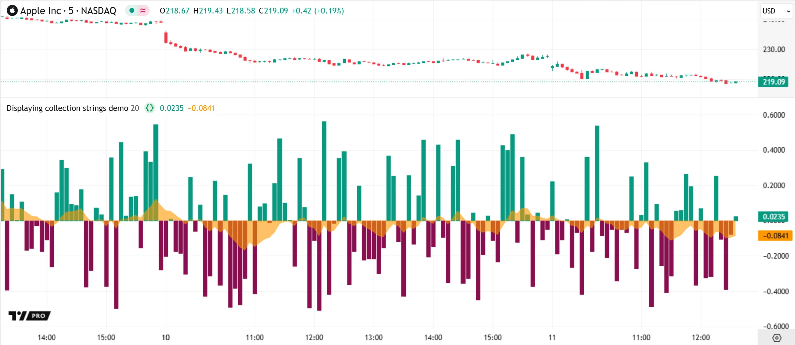
The following script calls request.security_lower_tf() to retrieve a “float” array containing close prices for each lower-timeframe bar within the current chart bar, which it uses to calculate an average intrabar price. Then, it calculates the ratio of the difference between the bar’s price and the intrabar average to the bar’s total range. The script plots the resulting ratio and its EMA in a separate pane:

To verify the ratio’s calculations, we can inspect the data stored in the intrabarPrices array by converting it to a “string” value and displaying the result for each bar.

The script version below declares a debugText variable that holds a formatted string representing the intrabarPrices array, the array’s size, and the avgPrice value. The script calls the log.*() functions to display the debugText value for each bar in the Pine Logs pane:

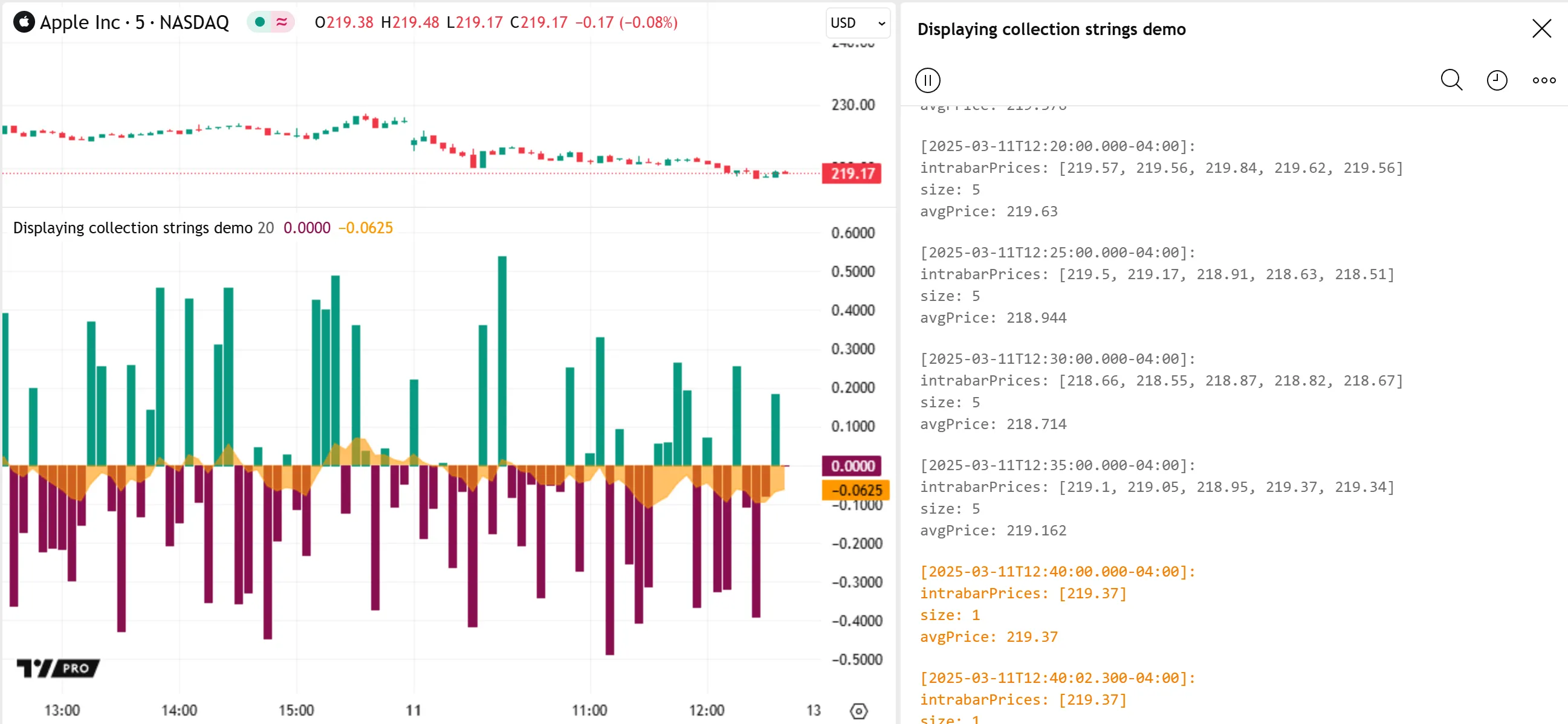
Note that:

• The script calls log.info() on confirmed bars and log.warning() on the open bar. Users can filter the logs by logging level to inspect confirmed and unconfirmed bars’ logs separately.
• For larger collections whose “string” representations exceed 4096 characters or cause excessive memory use, programmers can split them into smaller parts and convert them to strings separately. Alternatively, they can inspect individual elements via the *.get() method or for…in loops.

Inspecting individual elements

Collections of “color” or non-fundamental types (e.g., labels) do not have built-in “string” representations. Consequently, the technique described in the Displaying collection strings section does not work for them.

To inspect a collection that does not have a built-in “string” format, programmers can retrieve elements individually within for…in loops or using methods such as *.get(), then use those elements in custom “string” constructions or other output routines.

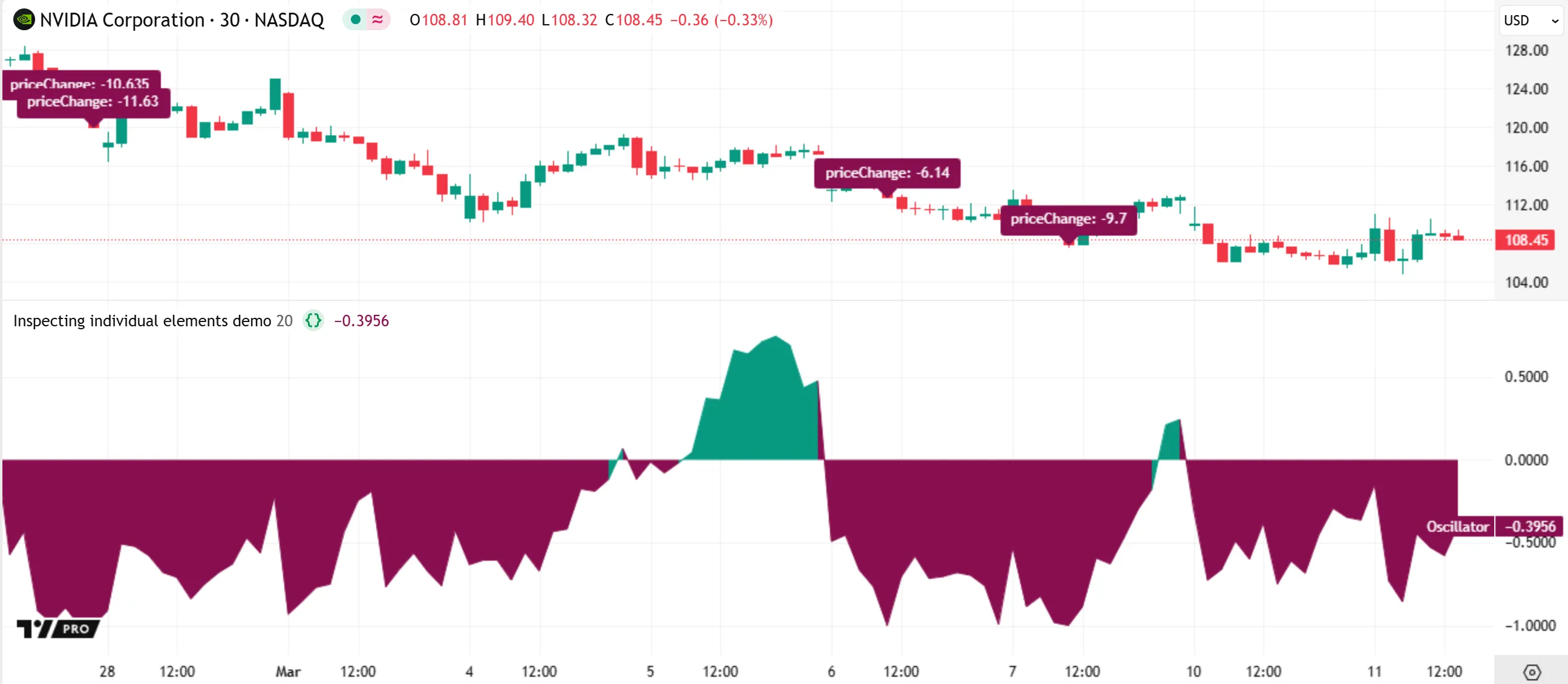
Consider the following example, which calculates the ratio of close changes to the overall close range over lengthInput bars. It plots the resulting osc in a separate pane, and it draws a label on the main chart pane each time the variable’s absolute value is 1:

When a script creates labels, it automatically maintains an array containing each active label’s reference. Programmers can access this array using the label.all variable, and thus inspect each individual label’s properties on any bar.

In the version below, the script executes a log.info() call to display the current bar_index and the size of the label.all array for the latest bar. Then, it iterates through the array with a for…in loop. On each iteration, the script calls log.info() to log formatted text containing the array index and the corresponding label’s x, y, and text properties. Additionally, the script plots the oldest and newest active labels’ y-coordinates on each bar:

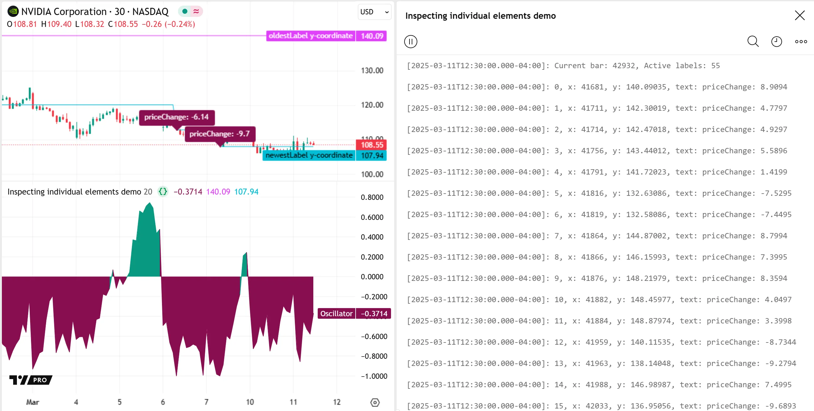
Note that:

• It is not possible to obtain all properties from drawing objects. For example, there is no built-in method to retrieve a label’s color. Some other types, such as table, do not have *.get_*() methods. If an object’s properties are not directly accessible, programmers can create separate variables for the arguments of the drawing’s *.new() or *.set_*() function, and then use those variables for debugging.
• In the above image, the logs show that the label.all array contains 55 elements. By default, Pine limits the number of labels to approximately 50, but the precise number of active labels varies. Programmers can increase the label drawing limit using the max_labels_count parameter of the indicator() or strategy() declaration statement.

Debugging objects of UDTs

User-defined types (UDTs) define the structures of objects. Objects contain a fixed set of fields, where each field can hold a separate value or reference to another specified type, even to another instance of the same user-defined type.

Because UDT objects can organize values and references to an arbitrary number of various different types, Pine does not have a built-in method to convert UDT objects to strings. Instead, to debug these structures, programmers must retrieve data from each field that requires inspection.

The following example defines a custom Data type with three fields. The first two fields reference arrays that hold successive price and time values. The third field specifies the number of bars between each new data sample. The script creates a new object of this type with a randomized length field on the first bar, then updates its arrays on bars whose bar_index values are divisible by that field.

The script uses array.covariance() and array.variance() on the object’s prices and times arrays to calculate a time-based slope of the collected data, and then plots the result on the chart:

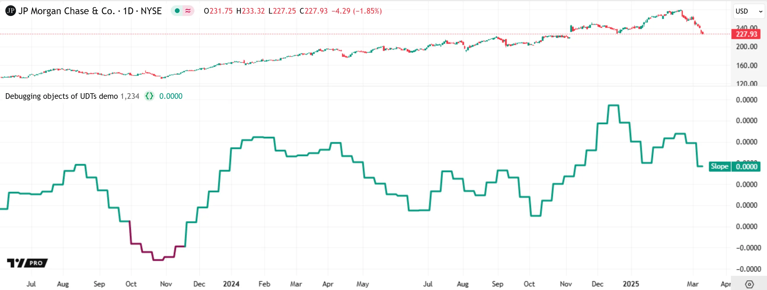
To verify and understand the script’s calculations, we can extract information from the Data object’s fields and inspect the data with Pine Logs or other outputs.

The script version below includes a log.info() call inside the if structure. The call displays formatted text representing information from the Data object’s prices, times, and length fields in the Pine Logs pane. Now, we can view each change to the object’s data to confirm the script’s behavior:

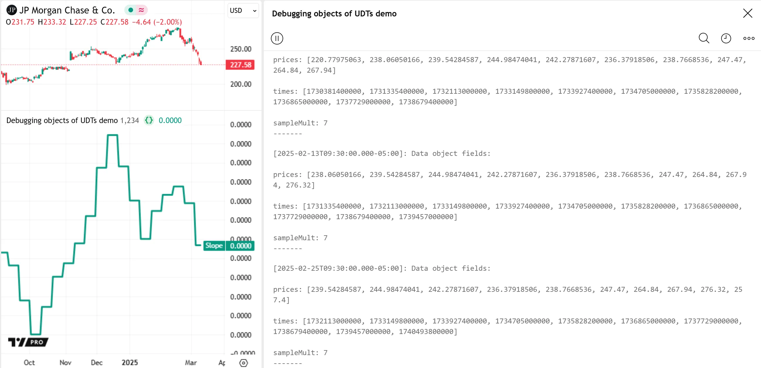
Note that:

• The script calls log.info() on confirmed bars and log.warning() on open bars, allowing users to filter the results by logging level in the Pine Logs pane.

Organization and readability

Source code that is organized and easy to read is typically simpler to debug. Furthermore, well-written code is more straightforward for programmers to maintain and improve over time. Therefore, we recommend prioritizing organization and readability throughout the script-writing process, especially while debugging.

Below are a few helpful coding recommendations based on our Style guide and best practices:

• Follow the script organization guidelines. Organizing scripts based on this structure makes different parts of the code simple to locate and inspect.
• Use identifiers that you can read, distinguish, and understand. When a code contains unclear identifiers, it is often harder to debug efficiently. See our Naming conventions to learn our recommended identifier format.
• Use type keywords to signify the qualified types that variables and parameters can accept. Although Pine can usually infer variable and parameter types, declaring them explicitly improves readability and helps programmers distinguish between assignment and reassignment operations. Plus, it enables Pine’s autosuggest feature to display more relevant type-based suggestions.
• Document the code using comments and compiler annotations (//@function, //@variable, etc.). The Pine Editor’s autosuggest displays the text from annotations when the mouse pointer hovers over identifiers, making it simple to recall what different parts of the code represent.